Volatility forecasting is a core task in quantitative finance, crucial for risk management, option pricing, and asset allocation. Among various models used for this purpose, GARCH (Generalized AutoRegressive Conditional Heteroskedasticity) models stand out due to their efficiency and effectiveness in capturing volatility patterns. In this article, we'll explore how to use GARCH models for volatility forecasting using the statsmodels library in Python.
Understanding GARCH Models
GARCH models are designed to model time series data where there is heteroskedasticity or variance changes over time. Created by Robert Engle in 1982, the ARCH model was extended by Tim Bollerslev in 1986 to the GARCH model, which can provide a more parsimonious representation in many financial time series.
The GARCH model specifies the variance of the current error term to be a function of the variances of the previous periods' error terms. Essentially, it takes past variances into account when predicting current volatility, making it extremely useful for financial data.
Setting Up the Environment
Before diving into the implementation, make sure you have Python installed along with necessary libraries, including statsmodels, numpy, and pandas. You can install these packages if they are not already available:
pip install numpy pandas statsmodelsData Preparation
For this tutorial, we'll use historical stock data. You can acquire such data using various sources like yfinance for stocks or other financial packages. Here’s an example of loading data for AAPL stock:
import pandas as pd
import numpy as np
import yfinance as yf

# Load historical data for Apple stock
data = yf.download('AAPL', start='2020-01-01', end='2023-01-01')

data['Return'] = np.log(data['Close'] / data['Close'].shift(1))
data.dropna(inplace=True)
Implementing GARCH Model
Once we have the returns computed, we can proceed to fit a GARCH model. The statsmodels library provides a robust framework to fit these models.
from statsmodels.tsa.arima.model import ARIMA
from arch import arch_model

# Fit the GARCH model
model = arch_model(data['Return'], vol='Garch', p=1, q=1)
model_fit = model.fit(disp='off')

print(model_fit.summary())
The above code snippet specifies a GARCH(1,1) model, which is the most commonly used variant. Here, p and q are orders representing the past squared returns and the lags of past variances that GARCH should include respectively.
Forecasting and Visualizing Volatility
Once the model is fitted, you can easily forecast volatility using the fitted model:
# Forecasting volatility
forecasts = model_fit.forecast(horizon=5)
print(forecasts.variance)
The horizon parameter specifies how many steps ahead you want to forecast the volatility. The output provides the forecasted variance, which can be visualized using plotting libraries such as matplotlib to better understand the results.
import matplotlib.pyplot as plt

plt.figure(figsize=(10, 4))
plt.plot(forecasts.variance[-1:], label="Forecasted Variance")
plt.title("Volatility Forecast")
plt.xlabel("Time")
plt.ylabel("Variance")
plt.legend()
plt.show()
Visualizing the forecasted volatility allows financial analysts to comprehend likely fluctuations in asset returns, better informing strategic decisions.
Conclusion
Using GARCH models with the statsmodels library provides a powerful way to forecast volatility in financial markets. These models help capture the time-dependent structures in variance, offering crucial insights for financial analysis and decision-making. While this introduction covers basic concepts and implementation, consider diving deeper into model extensions and testing your forecasts on various types of data to enhance predictive performance further.


