Introduction
Welcome to this comprehensive guide on using NumPy for signal processing. NumPy – which stands for Numerical Python – is one of the most essential libraries in Python for computational science, and it is especially useful for processing signals. We will explore how to leverage NumPy to manipulate and analyze signals that come in various forms such as sound, electromagnetic waves, and other time-varying phenomena.
The guide will start with basic concepts and then gradually level up to more advanced tactics. To gain the most benefit from this tutorial, the reader should have a basic understanding of Python programming and fundamental concepts of signal processing.
Getting Started
Before we dive into signal processing with NumPy, ensure you have the library installed. You can install it using pip:
pip install numpy
Let’s start by importing NumPy and checking its version:
import numpy as np
print(np.__version__)
Creating Signals in NumPy
First, we should know how to create signals. A simple way to generate a one-dimensional signal is by creating an array with specific frequencies. Here’s an example:
# Create a sample signal with a frequency of 5 Hz
t = np.linspace(0, 1, 500, endpoint=False)
y = np.sin(2 * np.pi * 5 * t)
Here, t is our time variable, with 500 samples taken over one second. The result y is a sine wave of 5 Hz.
Basic Operations on Signals
You can perform basic operations on signals such as scaling, shifting, and reversing
# Scaling the amplitude
y_scaled = 0.5 * y

# Shifting the signal
t_shifted = t + 0.5
y_shifted = np.sin(2 * np.pi * 5 * t_shifted)

# Reversing the signal
y_reversed = y[::-1]
Fourier Transform with NumPy
The Fourier Transform is essential in signal processing for frequency domain analysis. You can compute the Discrete Fourier Transform (DFT) using NumPy’s fft module:
# Compute the DFT of the signal
Y = np.fft.fft(y)
frequency = np.fft.fftfreq(t.shape[-1], d=t[1]-t[0])
We can plot the magnitude of the DFT:
import matplotlib.pyplot as plt
plt.plot(frequency, np.abs(Y))
plt.show()
Filtering
Filtering is a crucial process to remove unwanted parts from a signal. We will design a simple low-pass filter:
# Create a low-pass filter
def low_pass_filter(signal, cutoff_frequency, fs, order=5):
    nyquist = 0.5 * fs
    normal_cutoff = cutoff_frequency / nyquist
    b, a = scipy.signal.butter(order, normal_cutoff, btype='low', analog=False)
    filtered_signal = scipy.signal.filtfilt(b, a, signal)
    return filtered_signal
This example uses the scipy.signal module, which works well in conjunction with NumPy arrays.
Windowing
Windowing is used to minimize signal discontinuities at the boundaries before performing a Fourier Transform:
# Apply a Hanning window
window = np.hanning(len(y))
y_windowed = y * window
Noise Reduction
Noise can be reduced by averaging the signal, among other techniques:
# Moving average as a simple noise reduction technique
def moving_average(signal, n=3):
    ret = np.cumsum(signal, dtype=float)
    ret[n:] = ret[n:] - ret[:-n]
    return ret[n - 1:] / n
Signal processing with NumPy not only involves manipulating the data directly but also encompasses the usage of numerous supporting libraries such as SciPy, Matplotlib, and others that are designed to work well with NumPy arrays.
Conclusion
In conclusion, NumPy provides an extensive set of functionalities for signal processing, which can be utilized for a variety of applications. Whether you are scaling signals, filtering out noise, or applying Fourier transforms, NumPy serves as a powerful tool in the signal processing toolkit.
