How to Use Pandas for Geospatial Data Analysis (3 examples)

Introduction

Pandas, the go-to library for data manipulation in Python, also offers capabilities for handling geospatial data. This enables the analysis and visualization of geographical data within the familiar Pandas framework. In this article, we’ll explore how to leverage Pandas in conjunction with geospatial libraries to perform comprehensive geospatial data analyses through three practical examples.

Prerequisites

Before diving into the examples, ensure you have the following libraries installed:

• Pandas – for data manipulation
• Geopandas – an extension of Pandas for geospatial data operations
• Matplotlib – for data visualization
• GeoPy – a Python library for accessing geocoding services and performing location-based operations, such as distance calculations.

You can install these using pip:

pip install pandas geopandas matplotlib geopy

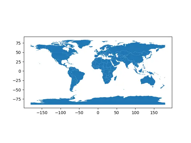
Example 1: Loading and Visualizing Geospatial Data

First, let’s start by loading geospatial data into a GeoDataFrame, which extends the functionalities of Pandas DataFrames for spatial data.

import geopandas as gpd

# Load geospatial data
world = gpd.read_file(gpd.datasets.get_path('naturalearth_lowres'))

# Preview the data
print(world.head())

# Plotting the world map
world.plot()
import matplotlib.pyplot as plt
plt.show()

Output (plot):

Output (print):

       pop_est      continent                      name iso_a3  gdp_md_est                                           geometry
0     889953.0        Oceania                      Fiji    FJI        5496  MULTIPOLYGON (((180.00000 -16.06713, 180.00000...
1   58005463.0         Africa                  Tanzania    TZA       63177  POLYGON ((33.90371 -0.95000, 34.07262 -1.05982...
2     603253.0         Africa                 W. Sahara    ESH         907  POLYGON ((-8.66559 27.65643, -8.66512 27.58948...
3   37589262.0  North America                    Canada    CAN     1736425  MULTIPOLYGON (((-122.84000 49.00000, -122.9742...
4  328239523.0  North America  United States of America    USA    21433226  MULTIPOLYGON (((-122.84000 49.00000, -120.0000...
2024-02-28 17:07:06.920 Python[56228:4438127] WARNING: Secure coding is not enabled for restorable state! Enable secure coding

This simple example demonstrates how to load geospatial data and plot a world map. Here, the world GeoDataFrame contains country boundaries which can be plotted directly using the plot method.

Example 2: Spatial Joins

Next, we focus on spatial joins.

import pandas as pd
import geopandas as gpd
from shapely.geometry import Point

# Sample data: Cities and their coordinates
data = {'City': ['New York', 'London', 'Tokyo'],
        'Latitude': [40.7128, 51.5074, 35.6895],
        'Longitude': [-74.0060, -0.1278, 139.6917]}
cities = pd.DataFrame(data)

# Convert DataFrame to GeoDataFrame
cities['Coordinates'] = list(zip(cities['Longitude'], cities['Latitude']))
cities['Coordinates'] = cities['Coordinates'].apply(Point)
cities_gdf = gpd.GeoDataFrame(cities, geometry='Coordinates')

# Spatial join with world GeoDataFrame
world = gpd.read_file(gpd.datasets.get_path('naturalearth_lowres'))
cities_in_world = gpd.sjoin(cities_gdf, world, how='inner', op='intersects')

print(cities_in_world.head())

Output:

Left CRS: None
Right CRS: EPSG:4326

  cities_in_world = gpd.sjoin(cities_gdf, world, how='inner', op='intersects')
       City  Latitude  Longitude                 Coordinates  ...      continent                      name iso_a3 gdp_md_est
0  New York   40.7128   -74.0060  POINT (-74.00600 40.71280)  ...  North America  United States of America    USA   21433226
1    London   51.5074    -0.1278   POINT (-0.12780 51.50740)  ...         Europe            United Kingdom    GBR    2829108
2     Tokyo   35.6895   139.6917  POINT (139.69170 35.68950)  ...           Asia                     Japan    JPN    5081769

[3 rows x 10 columns]

Spatial joins enable the merging of geospatial data based on spatial relationships. This example shows how you can map cities to countries by their geographic locations.

Example 3: Advanced Geospatial Analysis – Proximity and Distance Calculations

For our final example, we’ll dive into more advanced geospatial analyses, focusing on proximity and distance calculations.

from geopandas import GeoDataFrame
from shapely.geometry import Point, LineString
import geopy.distance

# Creating GeoDataFrame from coordinates
coords = [(0, 0), (1, 1), (2, 2), (3, 3)]
points = [Point(xy) for xy in coords]
gdf = GeoDataFrame(geometry=points)

# Calculating distances between points
for i in range(len(gdf) - 1):
    pt1 = gdf.loc[i, 'geometry']
    pt2 = gdf.loc[i + 1, 'geometry']
    distance = geopy.distance.geodesic((pt1.y, pt1.x), (pt2.y, pt2.x)).kilometers
    print(f'Distance between point {i} and {i + 1}: {distance} km')

Output:

Distance between point 0 and 1: 156.89956829134027 km
Distance between point 1 and 2: 156.87614940188664 km
Distance between point 2 and 3: 156.82932911607335 km

This example illustrates using the geopy library to calculate distances between points. This is particularly useful for analyzing the geographical spread of events or objects in space.

Conclusion

Through these examples, we’ve seen how Pandas can be used effectively for geospatial data analysis by leveraging libraries like Geopandas and matplotlib. Whether you’re looking to simply load and visualize spatial data, perform spatial joins, or conduct complex geographical analyses, the combination of these tools provides a powerful framework for geospatial data science projects.