Introduction
NumPy is a powerful library for numerical computing in Python. It provides support for arrays and matrices, along with a vast collection of mathematical functions to operate on these. This makes NumPy particularly well suited for scientific computing and complex numerical simulations.
In this tutorial, you will learn how to use NumPy to implement complex numerical simulations step by step. We will start with basic examples and gradually proceed to more advanced simulations.
Setting Up the Environment
Before we begin, you need to have Python and NumPy installed on your machine. You can install NumPy using pip:
pip install numpyNow, let’s start with some basics.
Basic NumPy Operations
To get started, let’s look at some simple matrix operations, which form the building blocks of most numerical simulations:
import numpy as np

# Creating two arrays
A = np.array([[1, 2], [3, 4]])
B = np.array([[5, 6], [7, 8]])

# Elementwise addition
C = A + B
print('Elementwise addition:\n', C)

# Matrix multiplication
D = np.dot(A, B)
print('Matrix multiplication:\n', D)
This will produce the following output:
Elementwise addition:
 [[ 6  8]
 [10 12]]
Matrix multiplication:
 [[19 22]
 [43 50]]
1D Harmonic Oscillator
Often, we begin with systems that are mathematically tractable and conceptually simple, such as a one-dimensional harmonic oscillator. The harmonic oscillator is a foundation for more complex physics. It’s described by the second-order differential equation:
m d^2x/dt^2 = -kxLet’s discretize time and simulate its motion over time using Euler’s method.
import numpy as np

# Constants
m = 1.0 # Mass of the oscillator
k = 1.0 # Spring constant

# Initial conditions
x = 1.0 # Initial displacement
v = 0.0 # Initial velocity

# Time stepping
dt = 0.1 # Time step
steps = 100 # Total number of steps to simulate

# Array to store displacements
x_values = np.zeros(steps)

for i in range(steps):
    a = -k/m * x
    v += a * dt
    x += v * dt
    x_values[i] = x

print(x_values)
This arrays of `x_values` now represents the oscillator’s displacement over the specified time frame.
Heat Equation
The next step up in complexity might be simulating the heat equation — a partial differential equation that describes the distribution of heat over time. For a one-dimensional rod, it is written as:
∂u/∂t = α ∂^2u/∂x^2To simulate this, we use a finite difference method.
import numpy as np
import matplotlib.pyplot as plt

# Parameters
alpha = 0.01
length = 10
num_points = 100

# Discretization
dx = length / num_points

# Initial condition (u at time 0)
u = np.sin(np.pi * np.linspace(0, length, num_points))
u[0] = 0 # Boundary condition at x=0
u[-1] = 0 # Boundary condition at x=L

dt = 0.01 # timestep
num_steps = 500

for _ in range(num_steps):
    du_dt = np.zeros_like(u)
    du_dt[1:-1] = alpha * (u[:-2] - 2*u[1:-1] + u[2:]) / dx**2
    u += du_dt * dt

plt.plot(np.linspace(0, length, num_points), u)
plt.show()
The plot generated by Matplotlib will show the temperature distribution along the rod after the specified time has passed.
Molecular Dynamics Simulation
For more advanced simulations, such as molecular dynamics, we have to iterate over many particles and time steps, accounting for their interactions. We will not delve into all the details here but rather set up a very simple scenario using NumPy arrays.
import numpy as np

# Suppose we have a system of 3 particles in 3 dimensions
positions = np.random.rand(3, 3)
velocities = np.zeros((3, 3))
timesteps = 1000
dt = 0.01

for _ in range(timesteps):
    # Compute forces between particles here
    # ...

    # Simple verlet integration (without the actual forces for brevity)
    new_positions = 2*positions - positions + forces*dt**2

    # Update positions
    positions = new_positions
This is an oversimplified snippet, the actual calculation of forces would depend on the system being modeled.
Conclusion
The examples provided here are just the tip of the iceberg when it comes to the complex simulations possible with NumPy. As your understanding grows, so too will the complexity of the problems you can tackle. The control and efficiency you gain from this power can significantly expand the scope of computational tasks you can undertake.
