NumPy: Get random samples from a multivariate normal distribution (3 examples)

Introduction

NumPy, a cornerstone library for numerical computing in Python, offers extensive functionality for random sampling, including the ability to generate samples from a multivariate normal distribution. Understanding this feature is essential for simulations, statistical modeling, and machine learning tasks where normality assumes a pivotal role.

Welcome to an exciting exploration of generating random samples from a multivariate normal distribution using NumPy. This journey not only enhances your data science toolkit but also dives into practical examples ranging from simple to complex applications.

What is a Multivariate Normal Distribution?

Before diving into code examples, let’s briefly understand the concept. A multivariate normal distribution is an extension of the univariate normal distribution to multiple dimensions, where each dimension represents a variable. It is characterized by mean vector and covariance matrix, dictating the distribution’s center and the correlation between variables, respectively.

Example 1: Basic Example

Let’s start with a basic example of generating random samples:

import numpy as np

# Parameters: mean vector and covariance matrix
mean = [0, 0]
cov = [[1, 0], [0, 1]]  # diagonal covariance, for independent variables

# Generate samples
samples = np.random.multivariate_normal(mean, cov, 5000)

print(samples)

This code generates 5000 samples from a two-dimensional normal distribution with mean [0,0] and an identity covariance matrix, implying independence and equal variance.

A possible output:

[[ 1.66083004  0.76686959]
 [-1.08087341  0.39214399]
 [-0.03251931  1.17903401]
 ...
 [ 0.39979638 -0.30943035]
 [-1.1714748   0.26815543]
 [-0.43391382  0.97492261]]

Example 2: Correlated Variables

Expanding on the first example, let’s see how to model correlated variables:

import numpy as np

# Parameters adjusted for correlation
mean = [0, 0]
cov = [[1, 0.5], [0.5, 1]]  # now there's correlation

# Generate samples
samples = np.random.multivariate_normal(mean, cov, 5000)

print("Samples with correlated variables:")
print(samples)

This snippet generates samples where the two variables have a positive correlation, as indicated by off-diagonal elements of the covariance matrix.

Possible output:

Samples with correlated variables:
[[-0.85891156  0.92035279]
 [-0.80370562  0.12568221]
 [ 0.75384196 -0.74140922]
 ...
 [-0.61681461 -0.91852092]
 [ 0.12062102 -0.34523382]
 [-0.90990227  0.27054913]]

Example 3: Higher Dimensions and Visualizing

Moving forward to more complex scenarios involves dealing with higher dimensions. Additionally, we’ll explore visualizing these samples:

import numpy as np
import matplotlib.pyplot as plt

# Define a higher-dimension mean and covariance
mean = [0, 0, 0]
cov = [[1, 0.5, 0.2], [0.5, 1, 0.3], [0.2, 0.3, 1]]  # higher-dimensional correlation

# Generate samples
samples = np.random.multivariate_normal(mean, cov, 5000)

# Visualization
fig = plt.figure(figsize=(10,7))
ax = fig.add_subplot(111, projection='3d')
ax.scatter(samples[:,0], samples[:,1], samples[:,2], c='blue', marker='o')
ax.set_title('3D Visualization of Multivariate Normal Samples')
plt.show()

Output (vary):

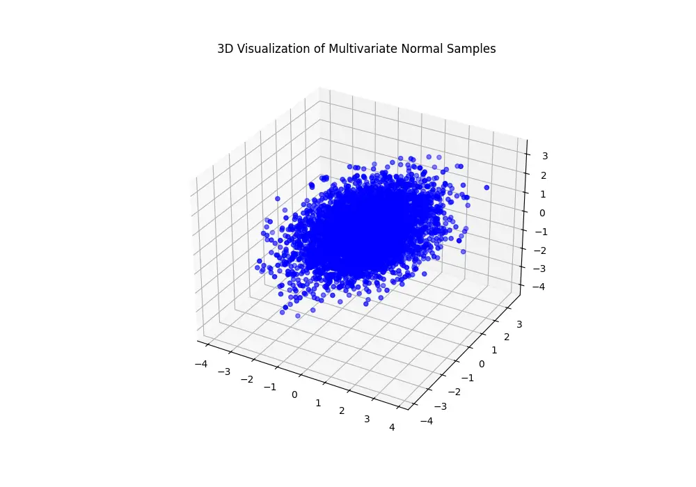
This example generates and visualizes samples from a three-dimensional multivariate normal distribution, showcasing how to handle more complex scenarios and the importance of visualization in understanding data distributions.

Conclusion

Sampling from a multivariate normal distribution in NumPy is a straightforward yet powerful tool for simulations, statistical analysis, and advanced modeling. Through the examples demonstrated, you should now have a good understanding of basic operations, dealing with correlations, and extending to higher dimensions. Embrace these techniques to enhance your data science and machine learning projects.