NumPy: Get samples from a negative binomial distribution (4 examples)

Overview

In this tutorial, we’ll explore how to use NumPy, a fundamental package for scientific computing with Python, to generate samples from a negative binomial distribution. This is particularly useful in various types of data analysis, simulations, and probabilistic modeling tasks. We’ll start with a basic understanding and move towards more advanced examples. By the end of this, you’ll have a solid grasp on generating and utilising negative binomial distributions in your projects.

The negative binomial distribution is a discrete probability distribution of the number of successes in a sequence of independent and identically distributed Bernoulli trials before a specified (non-random) number of failures occurs. It’s widely used in various fields such as ecology, quantum physics, and in processes that measure the number of failures before a success occurs.

Prerequisites

Before jumping into the examples, ensure you have the latest version of NumPy installed. You can install it using pip:

pip install numpy

Example 1: Basic Sample Generation

The first example demonstrates how to generate a simple sample from a negative binomial distribution using the numpy.random.negative_binomial function. This requires two parameters: n, the number of successes, and p, the probability of success in each trial.

import numpy as np

# Generate 10 samples with n=3 successes and p=0.5 probability of success
samples = np.random.negative_binomial(3, 0.5, 10)
print(samples)

This code will output a 1D array of 10 integers, each representing the number of failures before achieving the third success, based on a probability of success of 0.5 in each trial.

A possible output looks like this:

[1 1 0 5 2 0 3 2 3 0]

Example 2: Visualizing the Distribution

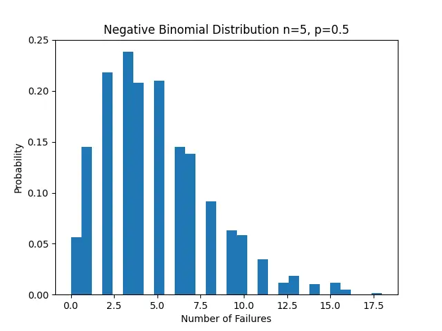
In the second example, we’ll dive deeper by visualizing the distribution of samples. This is a critical step in data analysis to understand the distribution’s shape and variability. We’ll use the matplotlib library for plotting. If you don’t have matplotlib installed, you can do so using:

pip install matplotlib

Code example:

import numpy as np
import matplotlib.pyplot as plt

n, p = 5, 0.5 # Number of successes and probability of success
samples = np.random.negative_binomial(n, p, 1000)

# Plotting
plt.hist(samples, bins=30, density=True)
plt.title('Negative Binomial Distribution n=5, p=0.5')
plt.xlabel('Number of Failures')
plt.ylabel('Probability')
plt.show()

This will produce a histogram visualizing the distribution of 1000 samples.

Output (vary):

Example 3: Modifying Parameters to See the Effect

Moving on to our third example, we’ll explore how changing the parameters n and p affects the distribution. Experimenting with different values for n and p can give us insights into the behavior of the distribution under various conditions.

import numpy as np
import matplotlib.pyplot as plt

# Experiment with different values of n and p
for n, p in [(3, 0.3), (10, 0.5), (5, 0.8)]:
    samples = np.random.negative_binomial(n, p, 1000)
    plt.hist(samples, bins=30, density=True, alpha=0.5, label=f'n={n}, p={p}')

plt.title('Varying n and p in Negative Binomial Distribution')
plt.xlabel('Number of Failures')
plt.ylabel('Probability')
plt.legend()
plt.show()

Result (vary):

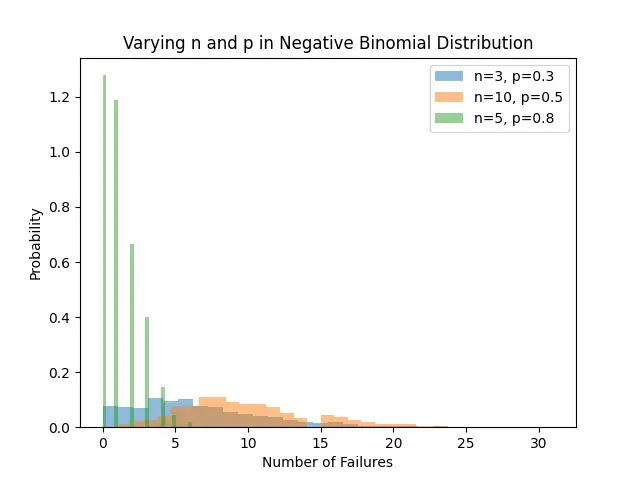
This code segment demonstrates the distribution patterns for different settings of n and p, providing a comparative insight.

Example 4: Advanced Application – Data Modeling

In our final example, we showcase an advanced application of the negative binomial distribution — data modeling. Let’s assume we are given a dataset where we suspect the data follows a negative binomial distribution due to the nature of the data collection process. Our goal is to fit a negative binomial model to this data.

import numpy as np
from scipy.stats import nbinom
import matplotlib.pyplot as plt

np.random.seed(2024)

# A big sample dataset
data = nbinom.rvs(10, 0.5, size=10000)

# Parameters estimation
mean_data = np.mean(data)
std_data = np.std(data)

# Estimate n and p
# This is simplified and for demonstration purposes. Real applications might require more sophisticated approaches.
n = mean_data ** 2 / (std_data ** 2 - mean_data)
p = mean_data / std_data ** 2

# Generate fitted model samples
fitted_samples = nbinom.rvs(n, p, size=1000)

# Visualization
plt.hist(fitted_samples, bins=30, density=True)
plt.hist(data, bins=30, density=True, alpha=0.5)
plt.title('Fitting Negative Binomial to Data')
plt.xlabel('Data Points')
plt.ylabel('Probability')
plt.show()

Output:

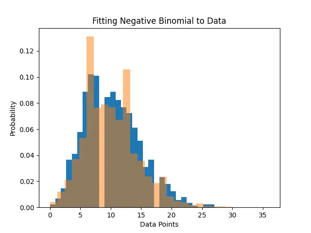
This example illustrates how the negative binomial distribution can be employed for modeling real-world data, offering a method to understand and characterize the distribution of data points.

Conclusion

Through these examples, we’ve explored the versatility and utility of the negative binomial distribution in analyzing and modeling data. Whether it’s understanding the basic generation process or applying it to complex data modeling scenarios, NumPy provides the tools necessary to handle this distribution efficiently. Mastery of these techniques will enhance your data analysis and probabilistic modeling skills, paving the way for deeper insights and more sophisticated analyses in your projects.