NumPy: Getting samples from geometric distribution (4 examples)

Introduction

NumPy, a fundamental package for numerical computing in Python, provides extensive support for working with arrays and matrices. Among its myriad of capabilities is the ability to generate samples from various statistical distributions, including the geometric distribution. In this tutorial, we will explore how to sample from a geometric distribution using NumPy, progressing from basic examples to more advanced scenarios.

The geometric distribution models the number of trials needed to achieve the first success in repeated Bernoulli trials. This distribution is useful in scenarios where one is interested in the likelihood of having to wait for an event to occur.

Example 1: Basic Sampling

Let’s start with the basics. To sample from a geometric distribution in NumPy, we use the numpy.random.geometric function:

import numpy as np

# The probability of success in a single trial
p = 0.5

# Generating a sample
sample = np.random.geometric(p, size=10)

print("Sample:", sample)

The p parameter represents the probability of success on a given trial, and size specifies the number of trials. The output would look something akin to this:

Sample: [1 3 2 1 2 2 4 1 2 1]

This output represents the trials needed to achieve the first success across 10 different experiments, based on a success probability of 0.5.

Example 2: Visualizing the Distribution

Understanding the distribution visually can often be as enlightening as analyzing the numbers. NumPy, coupled with Matplotlib, makes visualization straightforward:

import numpy as np
import matplotlib.pyplot as plt

# Generating a larger sample for a better distribution view
large_sample = np.random.geometric(0.35, size=1000)

plt.hist(large_sample, bins='auto', edgecolor='black')
plt.title('Histogram of Geometric Distribution')
plt.xlabel('Trials until first success')
plt.ylabel('Frequency')
plt.show()

Output (that changes each time you execute the code):

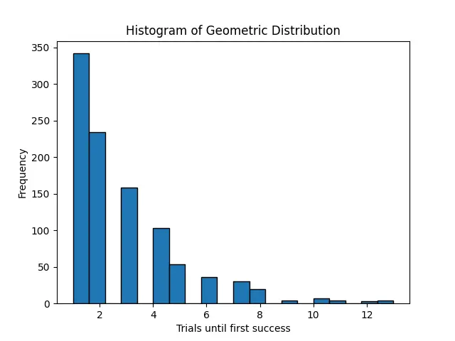
Here, we sampled 1000 experiments with a success probability of 0.35. The plotted histogram helps us understand the spread and central tendencies within our sampled geometric distribution.

Example 3: Varying Probabilities

In this example, we delve into how changing the success probability affects the geometric distribution:

import numpy as np
import matplotlib.pyplot as plt
import seaborn as sns

probabilities = [0.1, 0.3, 0.5, 0.7]

for p in probabilities:
    sample = np.random.geometric(p, size=1000)
    sns.distplot(sample, hist=False, kde=True, label=str(p))

plt.title('Geometric Distributions for Different Probabilities')
plt.xlabel('Trials until first success')
plt.ylabel('Density')
plt.legend()
plt.show()

Output (vary):

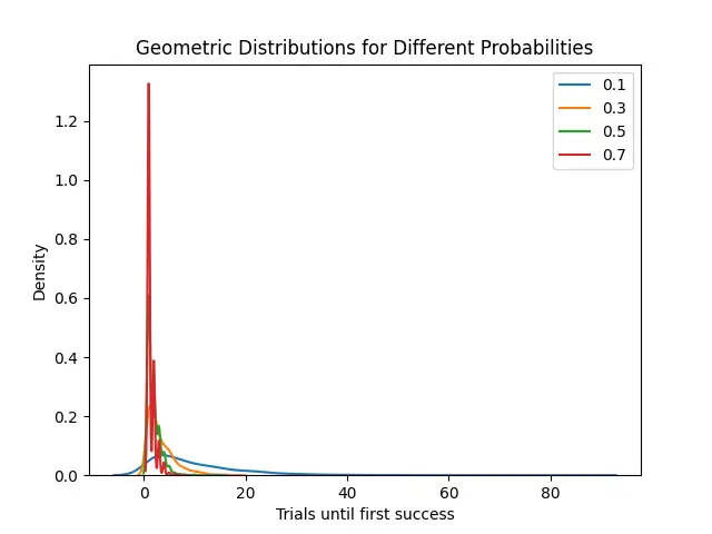
Utilizing Seaborn’s distplot, we plot the kernel density estimate (KDE) for each probability, providing a smoother representation of the distribution. This visualization elucidates how higher probabilities of success result in a distribution skewed towards fewer trials needed for the first success.

Example 4: Real-World Application – Network Connectivity

Let’s apply what we’ve learned to a practical problem. Consider a scenario where we want to model the number of attempts needed to establish a network connection, given that each attempt has a 20% success rate:

import numpy as np

# Assumption: 20% success rate for network connection attempts
p = 0.2
size = 10000

# Simulating the number of attempts until success
attempts = np.random.geometric(p, size=size)

# Calculating average based on simulated data
typical_attempts = np.mean(attempts)

print(f'Average number of attempts needed: {typical_attempts:.2f}')

Output (vary):

Average number of attempts needed: 5.01

This simulation can help network engineers understand, on average, how many attempts would be necessary before a successful connection. Such insights could be vital for planning, troubleshooting, and enhancing network performance.

Conclusion

Through this tutorial, we’ve explored various ways to generate and analyze samples from a geometric distribution using NumPy. Starting with basic sampling and progressing towards more elaborate examples, including visualization and application to real-world issues, provides a solid foundation for delving deeper into statistical modeling and data analysis with Python.