Overview
Understanding random data generation, especially with specific statistical distributions, is a fundamental skill in data science. NumPy, a core library for scientific computing in Python, offers an extensive toolkit for random number generation. Among its capabilities is the Generator.laplace() method, which allows for the generation of Laplace (or double exponential) distributed data. This tutorial explores the Generator.laplace() method through four examples, incrementally increasing in complexity, to guide you in effectively utilizing this tool in your data analysis workflows.
What is the Laplace Distribution?
The Laplace distribution, also known as the double exponential distribution, describes processes where events occur at a constant rate, but with possible deviations on both sides of a location parameter. The distribution is characterized by its location ( extmu) and scale ( extbeta) parameters. In the context of random number generation, employing the laplace() method allows simulations to mirror real-world phenomena encompassing these statistical properties.
Syntax & Parameters
Syntax:
generator.laplace(loc=0.0, scale=1.0, size=None)Here:
- loc: float or array_like of floats, optional. The position of the distribution peak. This is the “location” parameter. Default is
0.0. - scale: float or array_like of floats, optional. The exponential decay. This parameter dictates the “scale” of the distribution. Default is
1.0. - size: int or tuple of ints, optional. Specifies the output shape of the random samples. If not provided, a single value is returned. A tuple can specify a multi-dimensional array.
Example 1: Basic Usage of laplace()
First, let’s explore the most straightforward application of the Generator.laplace() method. To begin, you must import NumPy and initialize a random number generator.
import numpy as np
rng = np.random.default_rng()
Now, to generate five random numbers from a Laplace distribution with a location of 0 and a scale of 1:
laplace_data = rng.laplace(0, 1, 5)
print(laplace_data)
Each time you execute this code, it will produce a different set of five numbers due to the nature of random generation. However, they will always adhere to the Laplace distribution parameters specified. Below’s a possible output:
[-1.24761516 0.30607912 1.15947157 2.02182965 -0.12337132]Example 2: Visualizing Laplace Distribution
Moving beyond simple number generation, it’s insightful to visualize the distribution of a larger sample. This can help in understanding the spread and central tendency. Here’s how we can use Matplotlib, a powerful Python plotting library, to visualize the distribution:
import matplotlib.pyplot as plt
import numpy as np

rng = np.random.default_rng()


# Generating 1000 Laplace distributed numbers
data = rng.laplace(0, 1, 1000)

# Plot histogram
plt.hist(data, bins=30, density=True)
plt.title('Histogram of Laplace Distributed Data')
plt.xlabel('Value')
plt.ylabel('Frequency')
plt.show()
Output (vary):
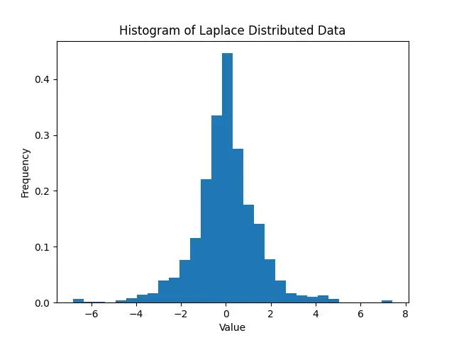
This histogram provides a visual snapshot of the generated data’s distribution, approximating the characteristic double-peaked contour of the Laplace distribution.
Example 3: Parametric Variations
The Generator.laplace() method’s flexibility allows for experimentation with different location and scale parameters. Observing how these modifications influence the output can be intriguing. In this example, we compare distributions with varying parameters.
import seaborn as sns
import matplotlib.pyplot as plt
import numpy as np

rng = np.random.default_rng()


# Generating data with different parameters
L1 = rng.laplace(0, 1, 1000)
L2 = rng.laplace(-5, 2, 1000)

# Plotting
sns.kdeplot(L1, label='Location=0, Scale=1')
sns.kdeplot(L2, label='Location=-5, Scale=2', linestyle='--')
plt.title('Density Plots of Laplace Distributions with Varied Parameters')
plt.legend()
plt.show()
Output (vary):
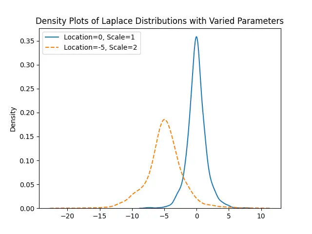
This approach highlights the impact of changing the location and scale on the distribution’s shape and spread. Using seaborn for plot enhancement makes the differences more discernible through smooth density plots.
Example 4: Application in Data Perturbation
Frequently, Laplace distributed noise is added to data as a method of perturbation, especially in mechanisms designed to preserve privacy like differential privacy. Let’s simulate the application of Laplace noise to a dataset:
import seaborn as sns
import matplotlib.pyplot as plt
import numpy as np

rng = np.random.default_rng()


# Original data - a simple array of ones
original_data = np.ones(1000)

# Generating Laplace noise
noise = rng.laplace(0, 1, 1000)

# Perturbed data
perturbed_data = original_data + noise

# Visualizing original vs perturbed data
plt.plot(noise, label='Laplace Noise', alpha=0.7)
plt.plot(perturbed_data, label='Perturbed Data', alpha=0.7)
plt.legend()
plt.title('Effect of Adding Laplace Noise to Data')
plt.show()
Output (vary):
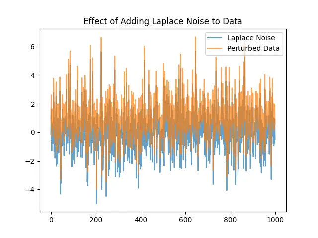
This example elucidates how Laplace distributed noise can introduce variation to a dataset, serving as a simplistic model for more complex data privacy techniques.
Conclusion
Through these examples, we’ve explored the versatility and utility of the Generator.laplace() method within NumPy’s random module. Understanding how to generate and employ Laplace distributed data is valuable across various scenarios, from data visualization to implementing privacy-preserving mechanisms in datasets. With NumPy’s comprehensive tools at your disposal, embracing the adept application of statistical distributions in Python becomes significantly more accessible.


