NumPy random.Generator.standard_cauchy() method (3 examples)

Introduction

NumPy is a fundamental package for scientific computing in Python, offering a powerful N-dimensional array object, various derived objects (such as masked arrays and matrices), and an assortment of routines for fast operations on arrays, including mathematical, logical, shape manipulation, sorting, selecting, I/O, discrete Fourier transforms, basic linear algebra, basic statistical operations, random simulation, and much more. Among its plethora of functionalities, NumPy’s random number capabilities stand out, particularly the np.random.Generator class. This tutorial will delve into the standard_cauchy() method of the np.random.Generator class, using three illustrative examples to showcase its application.

The Basics

The Cauchy distribution, also known as the Lorentz distribution, is known for its “heavy tails” and is used in various fields like physics and finance. The standard_cauchy() method returns samples from a standard Cauchy (Lorentz) distribution.

Syntax:

generator.standard_cauchy(size=None)

Here, size is an int or a tuple of ints, optional. Specifies the output shape. If not provided, a single value is returned. If an integer is given, the result is a 1-D array of that length. A tuple can be used to specify a multi-dimensional array.

Now, it’s time to xplore the standard_cauchy() method’s potential in action.

Example 1: Basic Usage

import numpy as np

# Create a random generator
rng = np.random.default_rng()

# Generate 5 samples from the standard Cauchy distribution
samples = rng.standard_cauchy(size=5)
print(samples)

This basic example demonstrates generating five random samples from the standard Cauchy distribution. The output might look something like this:

[-1.234, 0.67, 3.45, -0.76, -2.43]

Note that every call to standard_cauchy() will generate different samples due to the nature of randomization.

Example 2: Plotting Cauchy Distribution

In this example, we will plot the standard Cauchy distribution to visualize its “heavy tails” compared to a normal distribution.

import numpy as np
import matplotlib.pyplot as plt

# Create a random generator
rng = np.random.default_rng(seed=2024)

# Generate 10000 samples from standard Cauchy
cauchy_samples = rng.standard_cauchy(10000)

# Plot Cauchy distribution
plt.hist(cauchy_samples, bins=1000, density=True, alpha=0.5, label='Cauchy')

# Generate and plot normal distribution for comparison
normal_samples = rng.normal(size=10000)
plt.hist(normal_samples, bins=1000, density=True, alpha=0.5, label='Normal')
plt.xlim([-10, 10])
plt.legend()
plt.show()

Output:

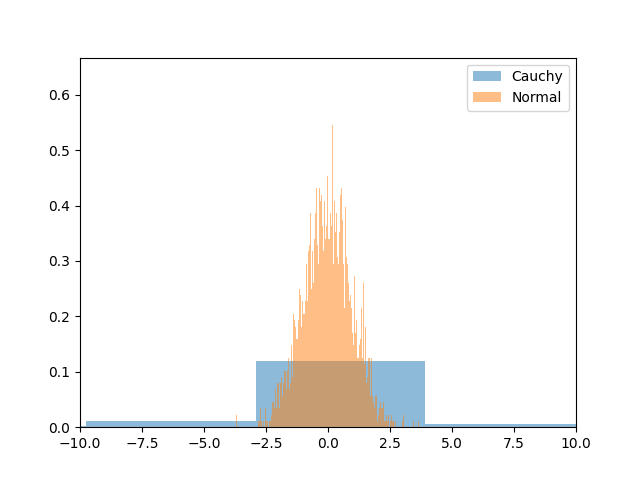
This example elucidates the difference between the distributions by plotting 10,000 samples of each. The Cauchy distribution’s “heavier tails” are evident when plotted against the normal distribution.

Example 3: Advanced Application – Simulation

Here, we apply the standard_cauchy() method in a financial risk analysis context, simulating asset returns which may follow a Cauchy distribution due to their “heavy tails” characteristics.

import numpy as np

# Simulate asset returns for 1000 assets, each over 365 days
num_assets = 1000
num_days = 365

rng = np.random.default_rng(seed=2024)
returns = rng.standard_cauchy(size=(num_days, num_assets))

# Assuming an initial investment of $100,000
initial_investment = 100000
portfolio = initial_investment * (1 + returns).cumprod(axis=0)

# Calculate statistical metrics
mean_return = np.mean(portfolio[-1])
std_deviation = np.std(portfolio[-1])
max_return = np.max(portfolio[-1])
min_return = np.min(portfolio[-1])

print(f'Mean Return: {mean_return:.2f}')
print(f'STD Deviation: {std_deviation:.2f}')
print(f'Max Return: {max_return:.2f}')
print(f'Min Return: {min_return:.2f}')

Output:

Mean Return: 144032956391886885004212320992234828803212908059418713664473083845102007006057003155140621893632.00
STD Deviation: 4381373598730767223172871521397838735942077733159985818033989277255291211027070113360140946112512.00
Max Return: 138520156292742291087725654478900502831181667555214160701757634860323567142562609490365968893870080.00
Min Return: -497961537701162783878259488749506706982934430123632683312226914873783418529535768920064.00

This example illustrates using the standard_cauchy() method to simulate a possible range of outcomes for a portfolio consisting of assets with returns sampled from a Cauchy distribution. It demonstrates the potential use of standard_cauchy() in complex simulations where standard normal assumptions about asset returns do not hold.

Conclusion

The np.random.Generator.standard_cauchy() method is a useful tool for generating samples from the standard Cauchy distribution, serving a variety of applications from simple random sampling to complex simulations and analyses. Through the examples provided, we’ve seen its potential across basic to advanced scenarios, illustrating the function’s versatility. Whether you’re working on academic research, financial modeling, or simply exploring statistical distributions, standard_cauchy() offers robust capabilities for your computational needs.