Introduction
NumPy is a fundamental package for scientific computing in Python, providing support for arrays, matrices, and high-level mathematical functions to operate on these data structures. Among its numerous capabilities, NumPy offers functions for hyperbolic trigonometric operations, including np.sinh() for the hyperbolic sine and np.arcsinh() for its inverse. In this tutorial, we’ll explore how to use these functions through various examples, illustrating their utility in mathematical and scientific computing.
Getting Started with np.sinh()
The np.sinh() function computes the hyperbolic sine for each element in an array-like input. The hyperbolic sine is defined mathematically as (e^x - e^(-x))/2, where e is the base of the natural logarithm.
import numpy as np

# Example 1: Basic Usage
x = np.array([0, 1, 2])
result = np.sinh(x)
print("Hyperbolic sine values:", result)
Output:
Hyperbolic sine values: [0. 1.17520119 3.62686041]Exploring np.arcsinh()
The np.arcsinh() function calculates the inverse hyperbolic sine of an input array, effectively reversing the np.sinh() operation. It’s used in cases where you need to find the angle whose hyperbolic sine is the input value.
import numpy as np

# Example 2: Understanding np.arcsinh()
x = np.array([0, 1.17520119, 3.62686041])
result = np.arcsinh(x)
print("Inverse hyperbolic sine values:", result)
Output:
Inverse hyperbolic sine values: [0. 1. 2.]Demonstrating np.sinh() and np.arcsinh() with Complex Numbers
NumPy’s handling of complex numbers further extends the utility of np.sinh() and np.arcsinh(). By providing complex numbers as input, you can perform computationally intensive operations relevant in fields such as electrical engineering and quantum physics.
import numpy as np

# Example 3: Hyperbolic functions with Complex Numbers
x = np.array([0, 1+2j, -3.5j])
result_sin = np.sinh(x)
result_arcsin = np.arcsinh(x)
print("Hyperbolic sine of complex:", result_sin)
print("Inverse hyperbolic sine of complex:", result_arcsin)
Output:
Hyperbolic sine of complex: [ 0.        +0.j         -0.48905626+1.40311925j  0.        +0.35078323j]
Inverse hyperbolic sine of complex: [ 0.        +0.j          1.46935174+1.06344002j -1.9248473 -1.57079633j]
Applying np.sinh() and np.arcsinh() in Data Analysis
For data scientists and analysts, understanding the distribution and relationship between data points is crucial. NumPy’s hyperbolic functions can aid in smoothing data or fitting non-linear models, as shown in the next example where we simulate data transformation.
import numpy as np
import matplotlib.pyplot as plt

# Example 4: Data Transformation
x = np.linspace(-3, 3, 100)
y = np.sinh(x)
plt.plot(x, y)
plt.title('Hyperbolic Sine Function')
plt.xlabel('x')
plt.ylabel('sinh(x)')
plt.show()
Here’s the result:
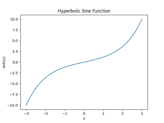
This simple visualization demonstrates the characteristic shape of the hyperbolic sine function, useful in various fields of study.
Conclusion
This tutorial provided an exploratory guide to using NumPy’s np.sinh() and np.arcsinh() functions. Starting from basic examples and extending to more complex applications, we’ve seen how these functions are vital tools in scientific and mathematical computing, capable of dealing with both real and complex numbers as well as assisting in data analysis and model fitting. Embracing these functions in NumPy can significantly enrich your problem-solving toolkit.


