NumPy – Using random.Generator.pareto() method (5 examples)

Introduction

This tutorial explores the random.Generator.pareto() method in NumPy, a powerful library for numerical computing in Python. The Pareto distribution, named after the economist Vilfredo Pareto, is a continuous distribution that is widely used in economics, finance, and many other fields for modeling phenomena where a small number of occurrences account for a large portion of the effect. Understanding how to generate Pareto-distributed random numbers can be crucial for simulations, random sampling, and modeling diverse phenomena.

Prerequisites

To follow along with this tutorial, you should have:

• A basic understanding of Python programming.
• NumPy installed. If not, you can install it using pip install numpy.

Example 1: Basic Pareto Distribution Sampling

First, let’s start with generating a simple Pareto distributed sample. This will help us understand the basics of using the random.Generator.pareto() method.

import numpy as np

# Initialize a random generator
rng = np.random.default_rng()

# Generate 10 samples with shape parameter a=3
samples = rng.pareto(a=3, size=10)
print(samples)

Output (vary):

[0.1028723  0.97859644 0.55975428 0.46357006 1.38884926 0.96426029
 0.16994503 0.13279623 0.21866431 1.00118415]

This will output an array of 10 numbers drawn from a Pareto distribution with a shape parameter (often denoted as alpha) of 3. The shape parameter significantly influences the distribution’s tail heaviness and overall shape.

Example 2: Plotting the Pareto Distribution

Next, we’ll plot the generated Pareto distribution samples to visually examine their distribution. This requires installing matplotlib, which can be done using pip install matplotlib, if not already installed.

import numpy as np
import matplotlib.pyplot as plt

# Initialize a random generator
rng = np.random.default_rng()

# Generate 10000 Pareto samples
samples = rng.pareto(a=3, size=10000)

# Calculate the histogram
count, bins, ignored = plt.hist(samples, bins=100, density=True, alpha=0.7, color='g')

# Plot the histogram
plt.title('Pareto Distribution (a=3)')
plt.show()

Output (vary):

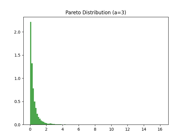
The histogram will reveal the characteristic “heavy-tailed” appearance of the Pareto distribution, with a small number of occurrences (samples in this case) accounting for most of the “weight” of the distribution.

Example 3: Pareto Distribution Properties: Mean and Variance

Understanding the mean and variance of a distribution is crucial for its application. The Pareto distribution has an interesting property where the mean and variance can drastically differ based on the shape parameter a.

import numpy as np


# Initialize a random generator
rng = np.random.default_rng()

# Import the necessary function
from scipy.stats import pareto

# Calculate the mean and variance
a = 3
mean, var = pareto.stats(a, moments='mv')
print(f'Mean: {mean}, Variance: {var}')

Output:

Mean: 1.5, Variance: 0.75

This will output the mean and variance for the Pareto distribution with a shape parameter of 3. Note that the scipy.stats module is used here for its convenience in statistical calculations.

Example 4: Application in Real-World Data

One of the primary applications of the Pareto distribution is in modeling wealth distribution within a population. Let’s simulate a scenario where we generate a hypothetical wealth distribution for 10,000 individuals.

import numpy as np
import matplotlib.pyplot as plt

# Initialize a random generator
rng = np.random.default_rng()

# Generate a wealth distribution sample
wealth_distribution = rng.pareto(a=2.5, size=10000) + 1

# Plot the wealth distribution
plt.hist(wealth_distribution, bins=100, color='blue', alpha=0.7)
plt.title('Simulated Wealth Distribution')
plt.show()

Output (vary):

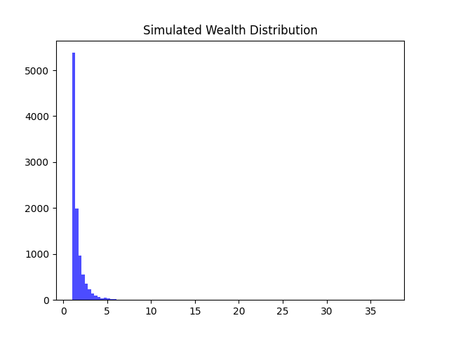
This histogram simulates a scenario where a small number of individuals hold most of the wealth, a common observation in real-world economies.

Example 5: Advanced Usage: Generating Custom Pareto Distributions

For more specialized applications, it might be necessary to generate Pareto distributions that do not align perfectly with standard parameters. By adjusting scale and location parameters, we can tailor distributions for specific needs.

import numpy as np
import matplotlib.pyplot as plt

# Initialize a random generator
rng = np.random.default_rng()

# Define custom parameters
a = 3.5
c = 2.0 # Scale parameter
location = 0.5 # Location parameter

# Generate the custom Pareto distribution
custom_pareto = c * (rng.pareto(a, size=10000) + 1) + location

# Plot the custom Pareto distribution
plt.hist(custom_pareto, bins=100, color='orange', alpha=0.7)
plt.title('Custom Pareto Distribution')
plt.show()

Output (vary):

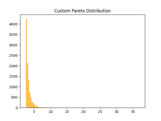
This advanced example demonstrates the flexibility of the random.Generator.pareto() method in generating distributions tailored to specific analytical or modeling needs.

Conclusion

The random.Generator.pareto() method in NumPy is a versatile tool for generating Pareto-distributed random numbers. Through this tutorial, we explored its basic usage, applications, and how to customize it for specific scenarios. Understanding and utilizing the Pareto distribution via NumPy can enhance simulations, data analysis, and modeling in various fields.