NumPy – Using random.Generator.power() method (4 examples)

NumPy is a core library for scientific computing in Python, providing a high-performance multidimensional array object and tools for working with these arrays. A key feature of NumPy is its ability to generate pseudo-random numbers for various statistical distributions, including the power distribution. In this tutorial, we’ll explore how to use the random.Generator.power() method in NumPy with four illustrative examples.

Understanding NumPy’s Power Distribution

Before delving into the examples, let’s briefly understand what the power distribution is and where it can be applied. The power distribution, also known as the Pareto distribution in certain contexts, is a probability distribution that follows a power-law. It is used in situations where large events are rare, but small events are common. These may include income distribution, file sizes on a computer, or sizes of natural phenomena.

The random.Generator.power() method generates samples from a power distribution characterized by a given shape parameter ‘a’. The method signature is as follows:

numpy.random.Generator.power(a, size=None)

Where ‘a’ is the shape parameter of the distribution and ‘size’ specifies the output shape.

Example 1: Generating a Simple Power Distributed Array

import numpy as np

# Initialize the random number generator
rng = np.random.default_rng(seed=2024)

# Generate an array of samples
samples = rng.power(a=3.0, size=1000)

print(samples)

This code snippet generates 1000 samples from a power distribution with a shape parameter of 3.0. The output is a one-dimensional NumPy array containing floating-point numbers that follow the specified power distribution.

Example 2: Plotting the Power Distribution

import numpy as np

# Initialize the random number generator
rng = np.random.default_rng(seed=2024)

# Generate an array of samples
samples = rng.power(a=3.0, size=1000)

import matplotlib.pyplot as plt

# Plot the distribution of the samples
plt.hist(samples, bins=50, density=True)
plt.title('Power Distribution (a=3.0)')
plt.show()

Output:

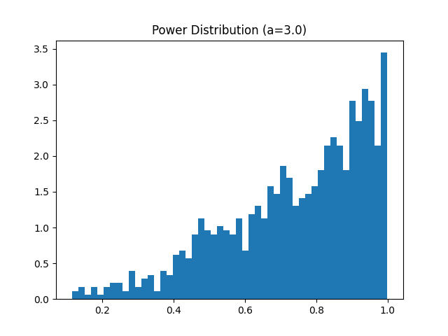
This example demonstrates how to visualize the power distribution of the generated samples. We use Matplotlib to create a histogram with 50 bins. The ‘density’ parameter is set to True to normalize the histogram, which lets us observe the shape of the power distribution more clearly.

Example 3: Generating Multidimensional Arrays

import numpy as np

# Initialize the random number generator
rng = np.random.default_rng(seed=2024)

# Generate a 2D array of samples
samples_2d = rng.power(a=5.0, size=(100, 10))

# Print the first 5 samples
print(samples_2d[:5])

In this third example, we generate a two-dimensional array of power distribution samples with a shape parameter of 5.0. The resulting array has 100 rows and 10 columns, demonstrating how the size parameter can be used to create multidimensional arrays.

Output (prints the first 5 samples only):

[[0.89489792 0.6410076  0.68935396 0.93804578 0.97976248 0.73089028
  0.83462846 0.81167778 0.60750611 0.91451897]
 [0.79733203 0.81233516 0.87518547 0.27245514 0.64459836 0.99802125
  0.99151867 0.82374871 0.81961295 0.58392441]
 [0.99056704 0.95757853 0.92352985 0.75693699 0.75064047 0.99387808
  0.80287961 0.79966471 0.64775239 0.91169484]
 [0.66951205 0.88887291 0.7244733  0.96329394 0.80128067 0.88544493
  0.5672985  0.5854202  0.64748523 0.99675838]
 [0.94950495 0.97246043 0.68102903 0.74632287 0.88550633 0.64581954
  0.42816404 0.96231634 0.46301036 0.71008891]]

Example 4: Using Power Distribution for Simulations

import numpy as np
# Scenario: Simulating the distribution of natural disaster damages

# Initialize the random number generator
rng = np.random.default_rng(seed=2024)

# Simulating disaster damages
a = 2.5  # Shape parameter
sizes = rng.power(a, size=1000) * 10000  # Scale the samples up

# Calculate and display summary statistics
mean_damage = np.mean(sizes)
std_damage = np.std(sizes)
print(
    f"Average Damage: ${mean_damage:.2f}\nStandard Deviation of Damage: ${std_damage:.2f}")

Output:

Average Damage: $7066.14
Standard Deviation of Damage: $2180.45

To demonstrate a practical application of the power distribution, this example involves simulating the distribution of damages from natural disasters, scaled up to represent monetary values. Using the power distribution with a shape parameter of 2.5, we generate 1000 samples to model the variability of damages. Summary statistics like the average and standard deviation provide insight into the simulated damages.

Conclusion

Through these examples, we’ve explored various ways to generate and use power-distributed data with NumPy’s random.Generator.power() method. From plotting distributions to simulating real-world phenomena, the flexibility and performance of NumPy’s random module offer powerful tools for statistical analysis and modeling. Understanding and applying these techniques opens up numerous possibilities for data analysis and scientific computing projects.