NumPy – Using random.Generator.weibull() method (5 examples)

Introduction

In this tutorial, we’re going to dive into the random.Generator.weibull() method provided by NumPy, a core library for numeric and scientific computing in Python. The Weibull distribution is a continuous probability distribution. It’s often used in reliability engineering and weather forecasting. Understanding how to generate Weibull-distributed random numbers can be vital for simulations and modeling in these and other fields.

The random.Generator.weibull() method draws samples from a two-parameter Weibull distribution. Its shape and scale parameters, denoted as a (shape) and b (scale), respectively, allow for diverse shapes of distributions useful in different contexts.

Syntax & Parameters

Syntax:

Generator.weibull(a, size=None, dtype=np.float64, out=None)

Parameters:

• a: The shape parameter of the Weibull distribution, a>0.
• size: Optional. An integer or tuple of integers, specifying the output shape. If the given shape is, for example, (m, n, k), then m * n * k samples are drawn. If size is None (default), a single value is returned.
• dtype: Optional. The desired data-type for the samples. The default data type is float64.
• out: Optional. An alternative output array in which to place the result. It must have a shape that the inputs broadcast to.

Returns:

• out: Samples from the Weibull distribution. If size is None, a single float is returned. Otherwise, a NumPy array of shape size is returned.

Example 1: Basic Use

import numpy as np

# Create a random generator instance
rng = np.random.default_rng()

# Generate 10 random numbers from a Weibull distribution with a=1.5
samples = rng.weibull(a=1.5, size=10)

print(samples)

Output (vary):

[0.70337024 1.04435918 1.52905732 1.27673546 0.73910972 0.64258335
 0.18957194 1.05974039 0.89978721 2.62364694]

The code snippet above demonstrates how to generate ten random numbers from a Weibull distribution. In this case, the shape parameter a is 1.5, creating a distribution that is slightly skewed to the right.

Example 2: Adjusting the Shape Parameter

import numpy as np

rng = np.random.default_rng()

# Generating numbers with different shape parameters
different_shapes = [rng.weibull(a, 1000) for a in [0.5, 1.0, 2.0, 5.0]]

for i, shape in enumerate(different_shapes):
    print(f"Shape {i}: mean = {np.mean(shape):.2f}, std = {np.std(shape):.2f}")

Output (vary):

Shape 0: mean = 2.13, std = 4.68
Shape 1: mean = 0.95, std = 0.91
Shape 2: mean = 0.89, std = 0.47
Shape 3: mean = 0.92, std = 0.21

By adjusting the shape parameter a, we can see how the characteristics of the generated distribution change. Lower values of a lead to distributions that emphasize lower numbers, while higher values skew the distribution towards higher numbers.

Example 3: Visualizing Distributions

import numpy as np
import matplotlib.pyplot as plt

rng = np.random.default_rng(seed=2024)

fig, ax = plt.subplots(1, 4, figsize=(20, 5))

for i, a in enumerate([0.5, 1.0, 2.0, 5.0]):
    data = rng.weibull(a=a, size=1000)
    ax[i].hist(data, bins=30)
    ax[i].set_title(f'Weibull distribution a={a}')

plt.tight_layout()
plt.show()

Output:

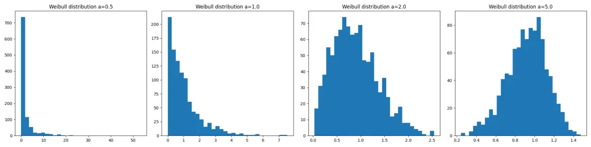
In this example, we employ matplotlib to visualize the effect of different shape parameters on the Weibull distribution. Through histograms, we can observe the distribution’s shape and how it changes as a varies. This visual aid is crucial for understanding the distribution’s nature in a more intuitive way.

Example 4: Comparing Weibull Distributions with Different Shape Parameters

This example compares Weibull distributions with different shape parameters to visualize how the shape parameter affects the distribution.

import numpy as np
import matplotlib.pyplot as plt

# Create a random generator instance
rng = np.random.default_rng(seed=2024)

# Shape parameters to compare
shapes = [0.5, 1.0, 1.5, 2.0, 5.0]
samples = 10000

# Generate samples and plot
plt.figure(figsize=(10, 6))
for a in shapes:
    data = rng.weibull(a, samples)
    plt.hist(data, bins=50, alpha=0.5, label=f'Shape={a}')

plt.title('Weibull Distributions with Different Shape Parameters')
plt.xlabel('Value')
plt.ylabel('Frequency')
plt.legend()
plt.show()

Output:

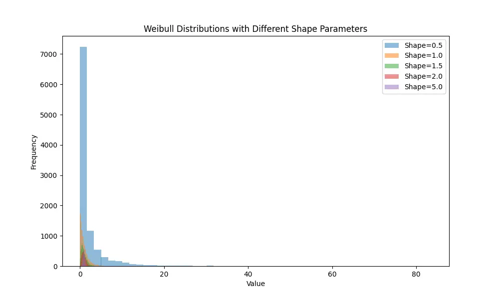
The code generates and plots histograms for Weibull distributions with different shape parameters, allowing us to observe the skewness and spread of the distributions as the shape parameter changes.

Example 5: Reliability Analysis Using Weibull Distribution

In this example, we simulate a reliability analysis scenario where the Weibull distribution is used to model the life of components. We’ll estimate the probability of failure before a certain time and plot the survival function.

import numpy as np
import matplotlib.pyplot as plt


def weibull_survival_function(a, b, t):
    """Calculate the survival probability using the Weibull survival function."""
    return np.exp(- (t / b) ** a)


# Parameters
a, b = 1.5, 1000  # Shape and scale
time = np.linspace(0, 2000, 1000)  # Time period

# Generate survival probabilities
survival_probabilities = weibull_survival_function(a, b, time)

# Plot
plt.figure(figsize=(10, 6))
plt.plot(time, survival_probabilities, label=f'Shape={a}, Scale={b}')
plt.title('Survival Probability over Time')
plt.xlabel('Time')
plt.ylabel('Survival Probability')
plt.legend()
plt.grid(True)
plt.show()

Output:

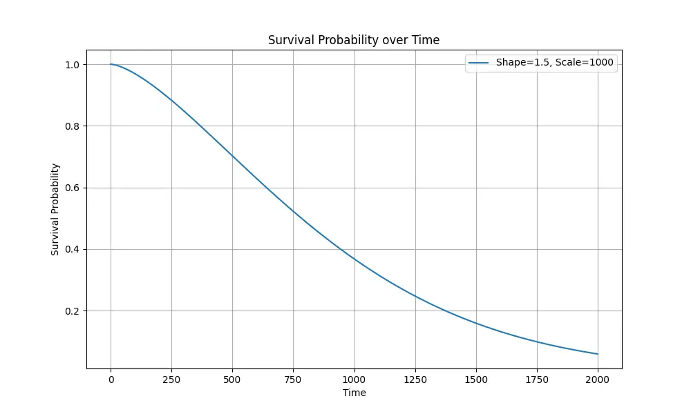
This code calculates and plots the survival function for a component with a given shape and scale parameter, illustrating how the probability of survival decreases over time. The survival function is crucial in reliability engineering for understanding and predicting the lifespan of components and systems.

Conclusion

This tutorial has traversed through the essentials of generating Weibull-distributed random numbers using NumPy’s random.Generator.weibull() method. Starting from basic generation, moving through manipulation of shape and scale parameters, and culminating in a practical example, we’ve explored how this method can be applied across various scenarios. By mastering these techniques, you can harness the power of simulation to model real-world phenomena accurately.