NumPy – Using random.Generator.rayleigh() method (4 examples)

NumPy is a fundamental package for scientific computing in Python. It offers a powerful N-dimensional array object and a plethora of functions for operating on these arrays. Among its many features, NumPy provides a comprehensive set of random number generators and functions for various statistical distributions, including the Rayleigh distribution. In this tutorial, we’ll explore the random.Generator.rayleigh() method through four illustrative examples, progressively increasing in complexity.

Introduction to Rayleigh Distribution

The Rayleigh distribution is often used in the field of signal processing and communications, particularly to model the magnitude of a randomly vector with Gaussian-distributed x and y components. Its probability density function is defined as:

f(x; \\sigma) = \frac{x}{\\sigma^2}e^{-x^2/(2\\sigma^2)}, for x \\geq 0

where \\sigma is the scale parameter, which defines the shape of the distribution.

Getting Started with random.Generator.rayleigh()

First, we need to import NumPy and create a random generator object:

import numpy as np

# Create a Generator object
rng = np.random.default_rng()

Example 1: Basic Usage

Generating a single number from the Rayleigh distribution is straightforward:

import numpy as np

# Create a Generator object
rng = np.random.default_rng()

# Generate a single Rayleigh-distributed number with a sigma of 2
number = rng.rayleigh(scale=2)
print(number)

This should output a float, which represents a number drawn from the Rayleigh distribution with specified scale parameter.

A possible output is:

1.4934698062909249

Example 2: Generating Multiple Numbers

Next, let’s generate an array of Rayleigh-distributed numbers:

import numpy as np

# Create a Generator object
rng = np.random.default_rng()

# Generate an array of 10 Rayleigh-distributed numbers
rayleigh_array = rng.rayleigh(scale=2, size=10)
print(rayleigh_array)

Output (vary):

[2.24991375 0.84062763 3.18748199 2.46631521 1.15632835 4.55513334
 4.21993572 1.56856714 2.42619047 1.84097204]

The size parameter allows us to specify the number of numbers to generate, resulting in an array of Rayleigh-distributed numbers.

Example 3: Visualization

Understanding data can be much smoother with graphical representations. Here, we’ll visualize a sample of 1000 numbers.

import numpy as np
import matplotlib.pyplot as plt


# Create a Generator object
rng = np.random.default_rng(seed=2024)

# Generate a large sample of Rayleigh-distributed numbers
large_sample = rng.rayleigh(scale=2, size=1000)

# Plotting
plt.hist(large_sample, bins=30, density=True)
plt.title('Histogram of Rayleigh-distributed Numbers')
plt.xlabel('Value')
plt.ylabel('Frequency')
plt.show()

Output:

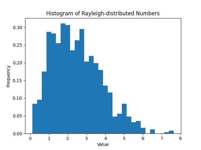
This histogram gives us a visual insight into the distribution of our Rayleigh-distributed sample.

Example 4: Application in Simulation

For a more advanced application, let’s use the Rayleigh distribution to model the envelope of a modulated signal with Gaussian noise. This can illustrate its utility in telecommunications engineering.

import numpy as np
import matplotlib.pyplot as plt

# Create a Generator object
rng = np.random.default_rng(seed=2024)

# Frequency and Time definitions
f = 100
T = 1.0 / 800.0

# Create a time vector
x = np.arange(0.0, 1.0, T)

# Creating a modulated signal
s = np.sin(2 * np.pi * f * x) + np.sin(2 * np.pi * 2 * f * x)

# Adding Rayleigh-distributed noise
gaussian_noise = rng.normal(0, 1, len(x))
rayleigh_noise = rng.rayleigh(scale=2, size=len(x))
signal_with_noise = s + gaussian_noise + rayleigh_noise

plt.plot(x, signal_with_noise)
plt.title('Modulated Signal with Rayleigh-distributed Noise')
plt.xlabel('Time')
plt.ylabel('Signal Amplitude')
plt.show()

Output:

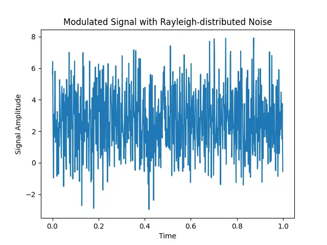
This simulation illustrates how Rayleigh-distributed noise can impact a signal, mimicking conditions that might occur in real-world telecommunications.

Conclusion

In this tutorial, we’ve taken a comprehensive look at the random.Generator.rayleigh() method in NumPy, from generating basic samples to applying the distribution in a complex simulation. Understanding the behavior of such distributions and their implementation can significantly advance analysis and simulations in scientific computing and engineering contexts. Harnessing NumPy’s powerful random number generation tools effectively opens doors to a multitude of applications in research and industry.