NumPy – Using random.Generator.standard_t() method (4 examples)

Introduction

NumPy is a cornerstone library in the Python ecosystem, extensively used for numerical computing. It provides a high-performance multidimensional array object, and tools for working with these arrays. An important subset of its vast functionality is NumPy’s random module, which has undergone improvements with the introduction of the random.Generator class, offering a more flexible and detailed approach to generating random numbers.

In this tutorial, we’ll explore the standard_t() method provided by the random.Generator class. This method samples from the standard Student’s t distribution with a specified degree of freedom. We’ll look at how this functionality can be used in various contexts through 4 examples, ranging from basic to advanced applications.

Syntax & Parameters

Syntax:

Generator.standard_t(df, size=None, dtype=np.float64, out=None)

Parameters:

• df: Degrees of freedom (ν). This must be a positive value.
• size: Optional. An integer or tuple of integers, specifying the output shape. If the given shape is, for example, (m, n, k), then m * n * k samples are drawn. If size is None (default), a single value is returned.
• dtype: Optional. The desired data-type for the samples. The default data type is float64.
• out: Optional. An alternative output array in which to place the result. It must have a shape that the inputs broadcast to.

Returns:

• out: Samples from the standard Student’s t-distribution. If size is None, a single float is returned. Otherwise, a NumPy array of shape size is returned.

Example 1: Basic Usage

To start with, let’s see how we can generate a single value from the standard t distribution:

import numpy as np

# Create a generator instance
rng = np.random.default_rng()

# Generate a single value with 10 degrees of freedom
value = rng.standard_t(10)
print(f'Single value: {value}')

Output (random):

Single value: -1.7792122283371132

This simple example shows the initial step in utilizing the standard_t() method. Notice how we first create a ‘rng’ instance of the random generator, which will be used to call our method.

Generating Multiple Values

Next, we will generate an array of values. This expands our initial demonstration to producing multiple outputs at once, showcasing how to simulate larger datasets:

import numpy as np

# Create a generator instance
rng = np.random.default_rng()

# Generate multiple values
values = rng.standard_t(10, size=100)
print(f'Array of values: {values}')

Output (random):

Array of values: [-1.12342809  1.0764163   1.44147345  1.45103538 -0.47478442 -0.32953218
  0.92406506  1.06296793 -0.1186412  -0.66017031 -2.14657269 -2.22936052
  2.01646282 -0.58923416 -0.23773015  0.22945822 -0.92062177  0.53834286
 -0.89075189 -1.19485289  0.26903464 -1.42874843  0.32252068  0.71700536
  0.43473835  1.2590101  -1.52440129 -1.66078544 -0.01746059  0.80182739
  1.0739121  -1.54043169  0.75498493 -0.3554167  -0.61934904  0.2728722
  0.88887874  1.18234084  0.34265018 -1.49492999  1.0266498   0.20835436
 -0.20249679  1.04482926 -0.5371166   1.08051742  0.59047968  0.51992327
 -0.53215359  0.33257253 -2.31715967  1.57336461 -0.4902499  -1.69413165
 -0.59373202  0.7268518  -0.24971074 -0.87011916 -0.88126651  0.79024643
 -0.24238987  0.76917403 -1.24331337 -0.12483328  0.87619646  0.83401762
  0.01667338 -0.90957513  0.32390409  2.41861039 -1.84779719 -1.68390199
 -1.58096434  0.82311155  0.01113392  0.86491868  0.14713461  1.13152564
 -0.70669096 -1.62863468  1.13548765 -0.82167219 -1.5312344  -1.84874136
 -0.40944981  0.90134347  0.4738103  -0.75779648 -0.32431097 -1.08767776
  0.18487957  1.7906035  -1.92995361 -1.33195605  2.2933643  -1.84910533
 -1.43370665  0.5284669   0.98689919  1.22358196]

This is a straightforward step towards conducting more extensive simulations or performing statistical analyses and model testing with generated data.

Distribution Visualization

For a more illustrative demonstration, we can visualize the distribution of generated values. This helps in understanding the shape and spread of the data we’re working with:

import matplotlib.pyplot as plt
import numpy as np

# Create a generator instance
rng = np.random.default_rng(seed=2024)


values = rng.standard_t(20, size=1000)
plt.hist(values, bins=30, edgecolor='black')
plt.title('Visualization of t Distribution')
plt.xlabel('Value')
plt.ylabel('Frequency')
plt.show()

Output:

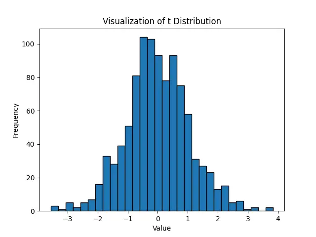
This visual approach helps in grasping the concept of the t-distribution, and how data might spread around the mean, especially when dealing with samples of different sizes.

Example 4: Advanced Data Simulation

Moving on to more advanced uses, we can simulate datasets for statistical experiments or research purposes. This example showcases generating a bivariate dataset with a specified correlation, using the t-distribution:

import numpy as np
import matplotlib.pyplot as plt

# Create a generator instance
rng = np.random.default_rng(seed=2024)

# Function to generate correlated data
def generate_data(degrees_of_freedom, size, correlation):
    x = rng.standard_t(degrees_of_freedom, size=size)
    y = correlation * x + \
        rng.standard_t(degrees_of_freedom, size=size) * \
        np.sqrt(1 - correlation ** 2)
    return x, y


# Generate dataset
x, y = generate_data(10, 1000, 0.5)

# Plot
plt.scatter(x, y)
plt.title('Simulated Correlated Data')
plt.xlabel('X')
plt.ylabel('Y')
plt.show()

Output:

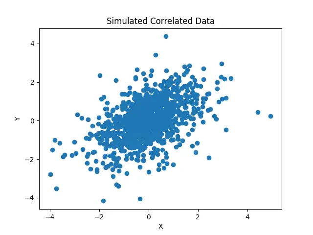
This example is indicative of the method’s robustness and versatility, allowing for complex simulations that contribute significantly to fields such as statistics and data science.

Conclusion

The standard_t() method from NumPy’s random.Generator class is a powerful tool for anyone involved in computational research, data analysis, or any field that requires an understanding and application of statistical distributions. Through these examples, ranging from basic usage to complex simulations, we’ve seen just how adaptable and invaluable this method can be.