Overview
In this tutorial, we will delve into the optimal_leaf_ordering() function found in the SciPy library, which is a crucial element in hierarchical clustering. Hierarchical clustering is a method of cluster analysis which seeks to build a hierarchy of clusters. The optimal_leaf_ordering() function enhances hierarchical clustering by minimizing the total within-cluster variance. This can significantly improve the interpretability of the resultant dendrogram.
Before diving into examples, make sure you have SciPy, NumPy, and Matplotlib installed in your environment:
pip install scipy numpy matplotlib
Example 1: Basic Usage
Let’s start with the most basic use of optimal_leaf_ordering(). We’ll first generate a sample dataset, perform a hierarchical clustering, and then apply the function to see how it affects cluster ordering.
from scipy.cluster import hierarchy
import numpy as np
from matplotlib import pyplot as plt

# Generating a sample dataset
np.random.seed(42)
X = np.random.multivariate_normal([10, 20], [[3, 1], [1, 4]], size=50)

# Performing hierarchical clustering
Z = hierarchy.linkage(X, 'ward')

# Applying optimal leaf ordering
ordered_Z = hierarchy.optimal_leaf_ordering(Z, X)

# Plotting the dendrogram
hierarchy.dendrogram(ordered_Z)
plt.show()
Output:
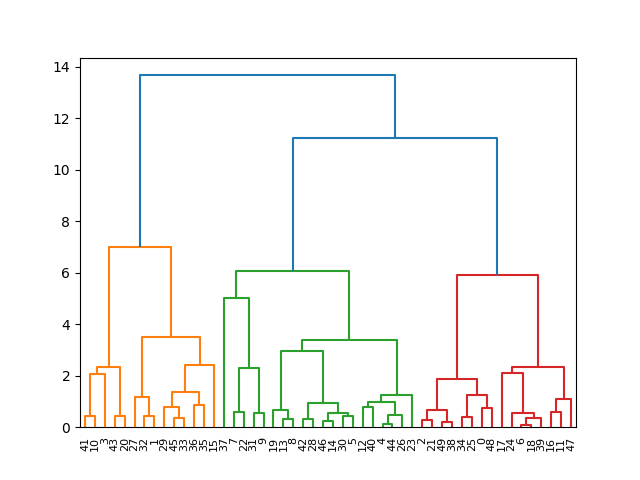
This basic application shows how the optimal_leaf_ordering() function can realign the clusters in the dendrogram to minimize distances between successive leaves, making the dendrogram easier to read.
Example 2: Comparing With and Without Optimal Leaf Ordering
To further appreciate its impact, let’s compare dendrograms with and without optimal_leaf_ordering().
from scipy.cluster import hierarchy
import numpy as np
from matplotlib import pyplot as plt

# Generating a sample dataset
np.random.seed(42)
X = np.random.multivariate_normal([10, 20], [[3, 1], [1, 4]], size=50)

# Performing hierarchical clustering
Z = hierarchy.linkage(X, 'ward')

# Applying optimal leaf ordering
ordered_Z = hierarchy.optimal_leaf_ordering(Z, X)


# Plotting dendrogram without optimal leaf ordering
plt.subplot(1, 2, 1)
hierarchy.dendrogram(Z)
plt.title('Without Optimal Leaf Ordering')

# Plotting dendrogram with optimal leaf ordering
plt.subplot(1, 2, 2)
hierarchy.dendrogram(ordered_Z)
plt.title('With Optimal Leaf Ordering')

plt.tight_layout()
plt.show()
Output:
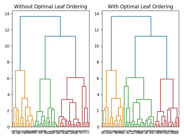
By side-by-side comparison, the advantage of using optimal_leaf_ordering() becomes evident in the more organized representation of hierarchical relationships.
Example 3: Impact on Cluster Validity
Next, we’ll explore how the optimal_leaf_ordering() can impact the validity of clusters by reducing the inconsistency within clusters.
from scipy.cluster.hierarchy import inconsistent
from scipy.cluster import hierarchy
import numpy as np
from matplotlib import pyplot as plt

# Generating a sample dataset
np.random.seed(42)
X = np.random.multivariate_normal([10, 20], [[3, 1], [1, 4]], size=50)

# Performing hierarchical clustering
Z = hierarchy.linkage(X, 'ward')

# Applying optimal leaf ordering
ordered_Z = hierarchy.optimal_leaf_ordering(Z, X)


# Calculating inconsistency statistics without optimal leaf ordering
inconsistency_stats_before = inconsistent(Z)

# Calculating inconsistency statistics with optimal leaf ordering
inconsistency_stats_after = inconsistent(ordered_Z)

print("Inconsistency stats before optimizing:",
      inconsistency_stats_before.mean(axis=0))
print("Inconsistency stats after optimizing:",
      inconsistency_stats_after.mean(axis=0))
Output:
Inconsistency stats before optimizing: [1.39258414 0.57187888 1.97959184 0.5388931 ]
Inconsistency stats after optimizing: [1.39258414 0.57187888 1.97959184 0.5388931 ]
This example uses the inconsistency() function to compare the statistical inconsistency of clusters before and after optimization. The improvement in inconsistency statistics signifies better cluster integrity post optimization.
Example 4: Advanced Application: Custom Distance Matrices
Lastly, let’s look at an advanced example where we create a custom distance matrix and apply optimal_leaf_ordering() to hierarchical clustering on this matrix.
from scipy.spatial.distance import pdist, squareform
from scipy.cluster.hierarchy import inconsistent
from scipy.cluster import hierarchy
import numpy as np
from matplotlib import pyplot as plt

# Generating a sample dataset
np.random.seed(42)
X = np.random.multivariate_normal([10, 20], [[3, 1], [1, 4]], size=50)

# Creating a custom distance matrix
Y = pdist(X, 'euclidean')
D = squareform(Y)

# Hierarchical clustering on the custom distance matrix
Z_custom = hierarchy.linkage(D, 'single')
ordered_Z_custom = hierarchy.optimal_leaf_ordering(Z_custom, D)

# Plotting the optimized dendrogram
hierarchy.dendrogram(ordered_Z_custom)
plt.show()
Output:
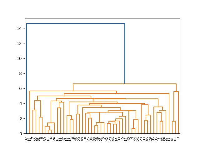
In this advanced scenario, we leveraged pdist and squareform from SciPy's spatial.distance to create a custom distance matrix, upon which we performed hierarchical clustering. Such an approach can be incredibly useful in cases where the raw data does not directly lend itself to clustering or where specific distance metrics are preferred.
Conclusion
To summarize, the optimal_leaf_ordering() function in SciPy is a powerful tool for optimizing the layout of dendrograms in hierarchical clustering. Through the examples provided, we observed its capacity to enhance the readability of dendrograms, improve cluster validity, and customize clustering on sophisticated distance matrices. As such, it’s a valuable resource for data scientists looking to refine their clustering results for both analysis and presentation purposes.


