SciPy cluster.vq.kmeans() function: Explained with examples

Introduction

Clustering is an unsupervised machine learning technique where we group a set of objects based on their similarity. Among various clustering algorithms, K-means is one of the most popular and simplest. The kmeans() function from SciPy is a powerful tool to perform K-means clustering. In this tutorial, we will cover how to use the kmeans() function comprehensively, illustrated with examples from basic to more advanced applications.

Basics of K-means Clustering

K-means clustering aims to partition n observations into k clusters in which each observation belongs to the cluster with the nearest mean, serving as a prototype of the cluster. The SciPy cluster.vq.kmeans() function provides a straightforward approach to achieve this. Before diving into coding examples, it’s critical to understand a few key concepts:

• Centroids: The center point of a cluster.
• Iteration: A single round of assigning points to the nearest centroid and updating the centroids’ positions.
• Convergence: The process ends when reaching a minimum value of the sum of the squared differences between points in a cluster and their respective centroid.

Setting up the Environment

Ensure you have SciPy installed in your Python environment. If not, you can install it using pip:

pip install scipy

Example 1: Basic K-means Clustering

We start with a basic example that creates a simple dataset and applies the kmeans() function.

import numpy as np
from scipy.cluster.vq import kmeans, vq

# Creating a dataset
data = np.array([[1, 1], [2, 1], [1, 0],
                 [4, 7], [3, 5], [4, 6]], dtype=np.float32)

# Applying kmeans
centroids, distortion = kmeans(data, 2)
print("Centroids:", centroids)

Output:

Centroids: [[1.3333334 0.6666667]
 [3.6666667 6.       ]]

This code snippet clusters our dummy dataset into two groups and returns the centroids of these groups. Notice how the centroids represent the mean location of points in each cluster.

Example 2: Determining the Optimal Number of Clusters

One of the challenges in K-means clustering is determining the optimal number of clusters. The elbow method is a common technique used to decide the appropriate number of clusters by plotting the sum of squared distances(SSD) versus the number of clusters.

We can use the kmeans() function to calculate SSD for various numbers of clusters and plot the results:

import numpy as np
from scipy.cluster.vq import kmeans
import matplotlib.pyplot as plt

# Generate artificial data
np.random.seed(123)
data = np.random.randn(300, 2)

# Calculate SSD for different numbers of clusters
SSD = []
for num_clusters in range(1, 11):
    centroids, distortion = kmeans(data, num_clusters)
    SSD.append(distortion)

# Plotting the Elbow graph
plt.plot(range(1, 11), SSD, 'bx-')
plt.xlabel('Number of clusters')
plt.ylabel('SSD')
plt.title('The Elbow Method showing the optimal number of clusters')
plt.show()

Output:

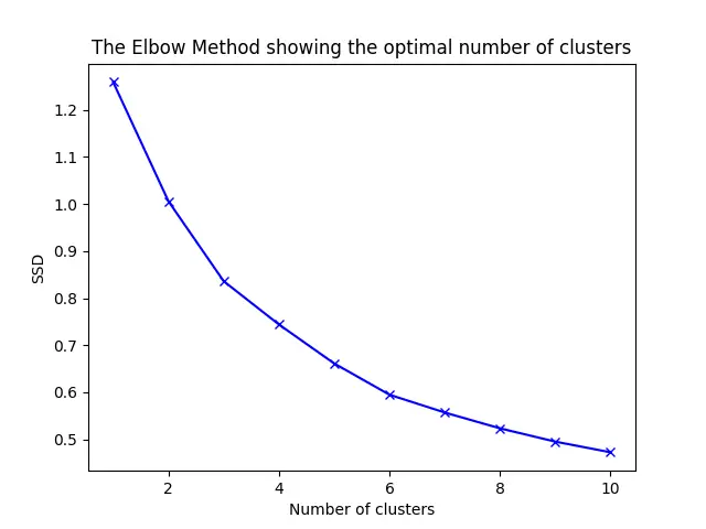
In the resulting plot, you should look for the “elbow” point, after which the reduction in SSD becomes less significant. This point suggests the optimal number of clusters for your dataset.

Example 3: Clustering with Feature Normalization

Before clustering, data normalization can significantly impact the results, especially when dealing with features of differing scales. Let’s demonstrate how to normalize features before applying kmeans().

import numpy as np
from scipy.cluster.vq import kmeans
from scipy.cluster.vq import whiten

data = np.array([[1, 400], [2, 800], [3, 200],
                 [5, 500], [7, 1000], [8, 600]])
data_normalized = whiten(data)

# appyling kmeans on normalized data
centroids, distortion = kmeans(data_normalized, 2)
print("Normalized Centroids:", centroids)

Output:

Normalized Centroids: [[2.9292505  3.06660751]
 [1.07405852 1.82079821]]

In whiten(), each feature is divided by its standard deviation across all observations, which results in features with a unit variance. This normalization makes the clustering process more efficient and accurate when features are on different scales.

Advanced Example: Image Color Clustering

One exciting application of K-means is image color clustering, where the goal is to find dominant colors in an image. Below is an example using the kmeans() function to cluster pixels based on their color values, effectively compressing the image’s color space into a few primary colors.

Before getting started, you need to install imageio:

pip install imageio

Here’s the code:

import numpy as np
from scipy.cluster.vq import kmeans
from imageio import imread, imsave
from sklearn.cluster import KMeans
import numpy as np

# Load image
image = imread('path_to_your_image.jpg')
# Preprocess the image data
pixels = np.reshape(image, (image.shape[0] * image.shape[1], image.shape[2]))
# Applying K-means
n_colors = 5
kmeans = KMeans(n_clusters=n_colors)
labels = kmeans.fit_predict(pixels)

# Reconstruct the image with the reduced palette
reconstructed_image = np.zeros_like(pixels)
for i in range(len(pixels)):
    reconstructed_image[i] = kmeans.cluster_centers_[labels[i]]
reconstructed_image = np.reshape(reconstructed_image, image.shape)

# Save the output image
imsave('compressed_image.jpg', reconstructed_image)

This advanced example illustrates how K-means can be applied beyond traditional numerical data, showcasing its flexibility and utility in real-world applications.

Conclusion

We have covered the basics through advanced usage of the cluster.vq.kmeans() function provided by SciPy, starting with simple clustering, determining optimal number of clusters, normalization of features, and even clustering image colors. This versatile function can be applied in numerous scenarios, proving to be an invaluable tool in your data science toolkit.