SciPy fft.idst() function (3 examples)

When diving into the realm of signal processing or working on relevant application projects, the importance of understanding transformations cannot be overstated. In particular, the Discrete Sine Transform (DST) and its inverse (IDST) are crucial tools for analyzing and processing signals.

The SciPy library, a mainstay for scientific computing in Python, offers a wide range of functions under its FFT (Fast Fourier Transform) module, one of which is fft.idst(), the function for inverse Discrete Sine Transform (IDST). This article aims to demystify this vital function through practical examples, aiding both beginners and advanced users in harnessing its power for signal processing tasks.

What is the IDST?

The Inverse Discrete Sine Transform (IDST) is the reverse operation of the Discrete Sine Transform (DST). While DST transforms a sequence of data points from the time domain to the frequency domain (sine components), IDST performs the opposite, converting the frequency-domain information back to the original time-domain sequence. This process is critical in applications where data restoration or signal reconstruction is necessary after frequency-domain manipulations.

Basic Example of Using fft.idst()

To initiate our journey into the fft.idst() function, let’s start with a simple example. This starting point will help beginners to grasp the basics of IDST.

from scipy.fft import idst
# Original sine wave frequencies
original_data = [0, 1, 0, -1]
# Applying IDST
reconstructed_data = idst(original_data, type=2)
print('Reconstructed data:', reconstructed_data)

Output:

Reconstructed data: [ 0.0517767  0.3017767 -0.3017767 -0.0517767]

This basic example demonstrates how to use the idst() function to reconstruct data points from their sine wave frequencies. The result is the original time-domain sequence, showcasing IDST’s capability to invert the DST process.

Advanced Example Involving Signal Processing

Building upon the basic example, let’s delve into a more complex scenario to illustrate the idst() function’s application in signal processing.

import numpy as np
from scipy.fft import idst, dst
# Generating a signal with multiple frequencies
freqs = [50, 75, 100]
sampling_rate = 500
T = 1 / sampling_rate
N = 1024
time = np.linspace(0, N*T, N, endpoint=False)
signal = np.sin(2 * np.pi * freqs[0] * time) + np.sin(2 *
                                                      np.pi * freqs[1] * time) + np.sin(2 * np.pi * freqs[2] * time)
# Applying DST and then IDST
dst_signal = dst(signal, type=2)
reconstructed_signal = idst(dst_signal, type=2)
print('Max difference between original and reconstructed signal:',
      np.max(np.abs(signal - reconstructed_signal)))

Output:

Max difference between original and reconstructed signal: 1.942890293094024e-15

This example demonstrates the process of signal reconstruction through IDST, after a signal containing multiple frequencies is first subjected to DST. The close similarity between the original and reconstructed signals, indicated by the minimal difference, highlights IDST’s accuracy and efficacy in real-world signal processing tasks.

Utilizing IDST in Image Processing

Moving beyond one-dimensional signals, the idst() function also finds applications in two-dimensional data scenarios such as image processing. This advanced example will showcase how IDST can be used for image rehabilitation.

from scipy.fft import idst
from matplotlib import pyplot as plt
from skimage import data
# Loading an example image
image = data.camera()
# Applying DST and then IDST on the image
fst_image = idst(image, type=2)
reconstructed_image = idst(fst_image, type=2)
# Displaying original and reconstructed images
plt.figure(figsize=(10, 5))
plt.subplot(1, 2, 1)
plt.imshow(image, cmap='gray')
plt.title('Original Image')
plt.subplot(1, 2, 2)
plt.imshow(reconstructed_image, cmap='gray')
plt.title('Reconstructed Image')
plt.show()

Output:

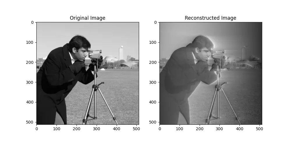
This exploratory step into the realm of image processing illustrates the versatility of the idst() function. By applying IDST to images, one can achieve tasks such as noise reduction, data compression, or even image restoration, showcasing the power of IDST across various data dimensions.

Conclusion

The fft.idst() function in SciPy serves as a powerful tool for performing inverse Discrete Sine Transforms, a crucial operation in signal and image processing domains. Through the examples provided, from basic to advanced, we have seen its potential in reconstructing signals and images from their frequency-domain representations. Understanding and utilizing the fft.idst() function can significantly enhance your ability to handle signal processing tasks, proving its worth as an invaluable component of the SciPy library.