The scipy.interpolate.griddata() function is a powerful tool in the SciPy library, designed for interpolating unstructured data to a structured grid. This makes it particularly useful in fields such as data visualization, numerical simulation, and geometric modeling, where it’s often necessary to create a smooth approximation of scattered data points. In this tutorial, we will explore four examples that demonstrate the functionality and versatility of griddata() from basic usage to more advanced applications.
Introduction to Scipy.interpolate.griddata()
Before delving into examples, let’s discuss what griddata() does and why it’s important. Essentially, griddata() takes three mandatory arguments: points, values, and the points at which to interpolate. Points are the coordinates of the input data, values are the data values at these points, and the grid points are the coordinates where you want the interpolation to be computed. The function supports different methods of interpolation — ‘linear’, ‘nearest’, and ‘cubic’ — each suitable for different scenarios.
Example 1: Basic Interpolation
import numpy as np
from scipy.interpolate import griddata

# Sample data
x = np.linspace(0, 10, 100)
y = np.linspace(0, 10, 100)
X, Y = np.meshgrid(x, y)
Z = np.sin(X) * np.cos(Y)

# Points to interpolate
points = np.random.rand(100, 2) * 10
values = np.sin(points[:,0]) * np.cos(points[:,1])

# Perform interpolation
grid_z = griddata(points, values, (X, Y), method='linear')

# Print result (for demonstration, we'll print just a snippet)
print(grid_z[49:51, 49:51])
Result:
[[-0.22288949 -0.21410357]
 [-0.31854018 -0.31064701]]
This example demonstrates the most straightforward use of griddata(): interpolating scattered data to a regular grid using linear interpolation. Notice how the approximations give us a smooth surface over the grid.
Example 2: Using Different Interpolation Methods
Next, let’s explore how the choice of interpolation method affects the result. As mentioned, griddata() offers ‘linear’, ‘nearest’, and ‘cubic’ as interpolation options. For physics or mathematical simulations where higher accuracy is required near known data points, ‘cubic’ might be preferable. However, it requires more computational time compared to ‘linear’ and ‘nearest’.
import matplotlib.pyplot as plt

# Use the same dataset as Example 1

# Linear interpolation
grid_z_linear = griddata(points, values, (X, Y), method='linear')

# Nearest interpolation
grid_z_nearest = griddata(points, values, (X, Y), method='nearest')

# Cubic interpolation
grid_z_cubic = griddata(points, values, (X, Y), method='cubic')

# Visualize
plt.figure(figsize=(12, 4))
plt.subplot(131)
plt.imshow(grid_z_linear)
plt.title('Linear')
plt.subplot(132)
plt.imshow(grid_z_nearest)
plt.title('Nearest')
plt.subplot(133)
plt.imshow(grid_z_cubic)
plt.title('Cubic')
plt.show()
Output:
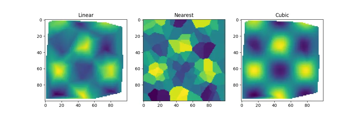
The visual comparison shows how ‘nearest’ tends to produce a blockier image, while ‘cubic’ offers a smoother surface, demonstrating the advantage of choosing the appropriate interpolation method based on the desired outcome.
Example 3: Deal With Out-of-Bounds Data
Handling data points outside the interpolation region is a common challenge. By default, griddata() assigns NaN (Not a Number) to these points, which can be problematic in some visualizations or analyses. You can address this by using the ‘fill_value’ argument to assign another value to these points.
# Using the dataset from the previous examples

# Perform interpolation with fill_value
grid_z_fill = griddata(points, values, (X, Y), method='linear', fill_value=0)

# Visualize
plt.figure()
plt.imshow(grid_z_fill)
plt.colorbar()
plt.title('Out-of-Bounds Handled with Zero')
plt.show()
Output:

This approach is invaluable when you need a complete dataset without NaNs for further processing or visualization.
Example 4: Interpolating Irregular Grids
Lastly, griddata() is not limited to rectilinear grids. You can interpolate data onto any grid configuration, including irregular grids. This is particularly useful in geographic applications where data conforms to features on the Earth’s surface rather than to a man-made grid.
# Define an irregular grid
theta = np.linspace(0, 2*np.pi, 100)
r = np.linspace(0, 10, 100)
T, R = np.meshgrid(theta, r)
x_irregular = R * np.cos(T)
y_irregular = R * np.sin(T)

# Interpolation
grid_z_irregular = griddata(points, values, (x_irregular, y_irregular), method='linear')

# Visualization
plt.figure()
plt.imshow(grid_z_irregular)
plt.colorbar()
plt.title('Interpolation on an Irregular Grid')
plt.show()
This example showcases the adaptability of griddata() to a wide range of applications, making it an invaluable tool in any data scientist’s toolkit.
Conclusion
The scipy.interpolate.griddata() function offers a versatile solution for interpolating scattered data to structured and unstructured grids. Through different interpolation methods and handling out-of-bounds data, it accommodates a broad set of requirements, ensuring smooth and accurate data approximation across various scientific and engineering fields.