SciPy interpolate.krogh_interpolate() function (4 examples)

SciPy’s krogh_interpolate() function is a powerful tool for polynomial interpolation. This function is particularly useful when you have a set of points through which you want to pass a smooth curve or when you are interested in estimating missing data points within a dataset. In this tutorial, we will explore how to use the krogh_interpolate() function through four detailed examples, ranging from basic usage to more advanced concepts.

What does Krogh Interpolation Mean?

Krogh Interpolation, also known as Hermite interpolation, offers a method to pass a polynomial of minimum degree through a given set of data points with potentially different x-values but unique corresponding y-values. This technique ensures that the resulting polynomial curve exactly fits the supplied data points, making it an invaluable tool in data analysis and scientific computing.

Example 1: Basic Krogh Interpolation

First, let’s start with a simple example. We will use krogh_interpolate() to fit a polynomial through a small dataset and evaluate the interpolated values at specific points.

import numpy as np
from scipy.interpolate import KroghInterpolator

x = np.array([0, 1, 2, 3])
y = np.array([1, 3, 2, 4])

interpolator = KroghInterpolator(x, y)
new_x = np.array([0.5, 1.5, 2.5])
interpolated_y = interpolator(new_x)

print("Interpolated values:", interpolated_y)

This code interpolates values at three new points (0.5, 1.5, and 2.5) based on the original dataset. The output will be the interpolated values at these points, illustrating how krogh_interpolate() can be used to predict values within the bounds of the given data.

Output:

Interpolated values: [2.75 2.5  2.25]

Example 2: Interpolating with Discontinuous Data

Now, let’s consider a scenario where the data has a discontinuity, such as a sudden jump in values. Krogh interpolation can still handle this effectively.

import numpy as np
from scipy.interpolate import KroghInterpolator

x = np.array([0, 2, 3, 4])
y = np.array([1, 2, 8, 4])  # Notice the jump from 2 to 8

interpolator = KroghInterpolator(x, y)
new_x = np.array([1, 2.5, 3.5])
interpolated_y = interpolator(new_x)

print("Discontinuity handled:", interpolated_y)

Output:

Discontinuity handled: [-3.75      5.609375  7.890625]

In this example, despite the discontinuity between 2 and 8, krogh_interpolate() effortlessly finds the appropriate polynomial that fits the data and extrapolates accordingly.

Example 3: Using Derivatives

A unique feature of Krogh interpolation is its ability to incorporate derivative information at the data points, providing a more accurate and tailored result based on known data behavior. Here’s how you could include first derivatives in your interpolation process.

import numpy as np
from scipy.interpolate import KroghInterpolator

x = np.array([0, 1, 2])
y = np.array([1, 3, 2])
derivatives = np.array([0, -1, 1])  # First derivatives at each point

interpolator = KroghInterpolator(x, (y, derivatives))
new_x = np.array([0.5, 1.5])
interpolated_y = interpolator(new_x)

print("Incorporating derivatives:", interpolated_y)

This example demonstrates how including derivatives can influence the shape of the interpolated polynomial, making the technique even more flexible and powerful.

Example 4: Handling Large-Scale Data

In this final example, we will scale up the process to handle larger sets of data, showcasing the robustness of the krogh_interpolate() function when dealing with substantial datasets.

import numpy as np
from scipy.interpolate import KroghInterpolator
import matplotlib.pyplot as plt

x = np.linspace(0, 10, 100)
y = np.sin(x) + 0.1 * np.random.rand(100)

interpolator = KroghInterpolator(x, y)
new_x = np.linspace(0, 10, 500)
interpolated_y = interpolator(new_x)

plt.plot(x, y, 'o', label='Data Points')
plt.plot(new_x, interpolated_y, '-', label='Interpolated Curve')
plt.legend()
plt.show()

Output:

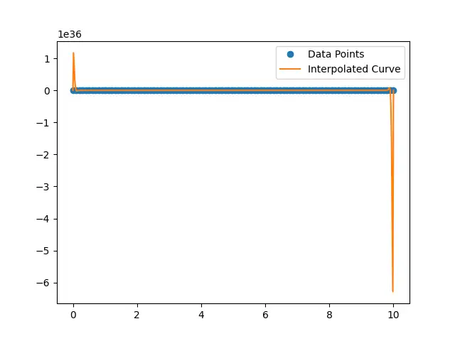
This time, incorporating random noise into our synthetic data simulates a more realistic dataset. The result is a smooth curve that captures the underlying trend of our noisy data, demonstrating how krogh_interpolate() acts in real-world applications.

Conclusion

In conclusion, the krogh_interpolate() function in SciPy is an incredibly versatile tool for polynomial interpolation. Throughout our examples, from basic interpolation tasks to incorporating derivative information and handling discontinuities and large-scale data, it demonstrates its capability to adapt and deliver precise interpolations. Whether you’re filling in missing data, approximating functions, or smoothing data points, krogh_interpolate() offers a reliable solution.