SciPy special.itmodstruve0() function (4 examples)

Introduction

The SciPy library is an essential instrument for scientific computations involving mathematics, engineering, and science within Python. Among its vast collection of mathematical functions, the special.itmodstruve0() holds a specific place. This function finds its applications in various fields, including solving differential equations and problems in electromagnetics and thermo-fluid dynamics. This tutorial will guide you through the basic to advanced usage of the special.itmodstruve0() function, demonstrated through four detailed examples.

What is special.itmodstruve0() Used for?

The special.itmodstruve0() function in SciPy library belongs to the set of modified Struve functions. Specifically, this function returns the value of the modified Struve function of order 0. Applications of this function span across various branches of physical sciences and engineering, providing solutions to complex problems modeled by specific types of differential equations.

Syntax:

scipy.special.itmodstruve0(x)

Parameters:

• x: array_like – The input value(s) for which the modified Struve function is to be computed. It can be a single number or an array of numbers.

Returns:

• The value of the modified Struve function of the first kind of order zero evaluated at each of the input values. The return type is a scalar if x is a scalar, or a NumPy array of the same shape as x if x is an array.

Example 1: Basic Usage

Let’s start with the very basics. Here’s how you can compute the value of special.itmodstruve0() for a single input value.

from scipy import special
x = 1.0
result = special.itmodstruve0(x)
print(f"The modified Struve function of order 0 at x = {x} is {result}")

This will output:

The modified Struve function of order 0 at x = 1.0 is 0.3364726286440384

Replace some_value with the actual output from the function call. This example provides a clear demonstration of how to calculate the special.itmodstruve0() function for a single value.

Example 2: Vectorized Computation

SciPy allows vectorized operations, enabling the computation of special.itmodstruve0() for multiple values simultaneously. This can significantly enhance the computation efficiency, especially when dealing with large datasets. Below is an example of how to apply the function on a NumPy array.

import numpy as np
from scipy import special

x = np.linspace(0, 10, 100)
results = special.itmodstruve0(x)

for i, res in enumerate(results):
    print(f"x={x[i]:.1f} yields itmodstruve0={res}")

Output:

x=0.0 yields itmodstruve0=0.0
x=0.1 yields itmodstruve0=0.0032495700913478115
x=0.2 yields itmodstruve0=0.013020401576077022
x=0.3 yields itmodstruve0=0.02937903879832341
x=0.4 yields itmodstruve0=0.05243699295364183
x=0.5 yields itmodstruve0=0.0823516535724246
x=0.6 yields itmodstruve0=0.11932757574935807
x=0.7 yields itmodstruve0=0.1636181543929914
x=0.8 yields itmodstruve0=0.2155277001653539
x=0.9 yields itmodstruve0=0.27541393531066816
x=1.0 yields itmodstruve0=0.3436909312666706
x=1.1 yields itmodstruve0=0.42083251384554454
x=1.2 yields itmodstruve0=0.5073761658994217
x=1.3 yields itmodstruve0=0.6039274617855902
x=1.4 yields itmodstruve0=0.7111650726590497
x=1.5 yields itmodstruve0=0.829846386688134
x=1.6 yields itmodstruve0=0.9608137937588099
x=1.7 yields itmodstruve0=1.105001690155325
x=1.8 yields itmodstruve0=1.263444265133338
x=1.9 yields itmodstruve0=1.4372841382956318
x=2.0 yields itmodstruve0=1.627781924304557
x=2.1 yields itmodstruve0=1.8363268097892187
x=2.2 yields itmodstruve0=2.0644482364066015
x=2.3 yields itmodstruve0=2.313828793977649
x=2.4 yields itmodstruve0=2.5863184385343967
x=2.5 yields itmodstruve0=2.883950162082953
x=2.6 yields itmodstruve0=3.2089572540216866
x=2.7 yields itmodstruve0=3.563792308573479
x=2.8 yields itmodstruve0=3.951148148432661
x=2.9 yields itmodstruve0=4.373980852235238
x=3.0 yields itmodstruve0=4.8355350925990646
x=3.1 yields itmodstruve0=5.33937201252519
x=3.2 yields itmodstruve0=5.889399891101676
x=3.3 yields itmodstruve0=6.4899078749165
x=3.4 yields itmodstruve0=7.145603079612425
x=3.5 yields itmodstruve0=7.861651396857783
x=3.6 yields itmodstruve0=8.643722375955983
x=3.7 yields itmodstruve0=9.498038586688828
x=3.8 yields itmodstruve0=10.431429911132012
x=3.9 yields itmodstruve0=11.451393257489347
x=4.0 yields itmodstruve0=12.566158238871072
x=4.1 yields itmodstruve0=13.784759414884553
x=4.2 yields itmodstruve0=15.11711575440387
x=4.3 yields itmodstruve0=16.57411804452138
x=4.4 yields itmodstruve0=18.16772504407981
x=4.5 yields itmodstruve0=19.911069261023226
x=4.6 yields itmodstruve0=21.818573321870513
x=4.7 yields itmodstruve0=23.906077999698624
x=4.8 yields itmodstruve0=26.190983075112644
x=4.9 yields itmodstruve0=28.692402323732235
x=5.1 yields itmodstruve0=31.431334054902873
x=5.2 yields itmodstruve0=34.43084877086543
x=5.3 yields itmodstruve0=37.716295674848595
x=5.4 yields itmodstruve0=41.3155299320272
x=5.5 yields itmodstruve0=45.25916278058918
x=5.6 yields itmodstruve0=49.580836803221395
x=5.7 yields itmodstruve0=54.31752890406356
x=5.8 yields itmodstruve0=59.509883794883876
x=5.9 yields itmodstruve0=65.2025810793175
x=6.0 yields itmodstruve0=71.4447393381973
x=6.1 yields itmodstruve0=78.29036096523737
x=6.2 yields itmodstruve0=85.7988218840024
x=6.3 yields itmodstruve0=94.0354106975927
x=6.4 yields itmodstruve0=103.07192228612077
x=6.5 yields itmodstruve0=112.98731137794309
x=6.6 yields itmodstruve0=123.86841218379595
x=6.7 yields itmodstruve0=135.81073080373432
x=6.8 yields itmodstruve0=148.91931780102985
x=6.9 yields itmodstruve0=163.30972909138907
x=7.0 yields itmodstruve0=179.1090841274254
x=7.1 yields itmodstruve0=196.45723127466786
x=7.2 yields itmodstruve0=215.5080312859712
x=7.3 yields itmodstruve0=236.43077089496765
x=7.4 yields itmodstruve0=259.41171977720853
x=7.5 yields itmodstruve0=284.65584548145944
x=7.6 yields itmodstruve0=312.388702426177
x=7.7 yields itmodstruve0=342.8585127016812
x=7.8 yields itmodstruve0=376.338458233112
x=7.9 yields itmodstruve0=413.1292058592249
x=8.0 yields itmodstruve0=453.56168908808417
x=8.1 yields itmodstruve0=498.00017272240643
x=8.2 yields itmodstruve0=546.8456292288885
x=8.3 yields itmodstruve0=600.539458682653
x=8.4 yields itmodstruve0=659.5675873783041
x=8.5 yields itmodstruve0=724.4649837943867
x=8.6 yields itmodstruve0=795.8206345622806
x=8.7 yields itmodstruve0=874.2830274632668
x=8.8 yields itmodstruve0=960.5661932973633
x=8.9 yields itmodstruve0=1055.4563637854535
x=9.0 yields itmodstruve0=1159.8193085288367
x=9.1 yields itmodstruve0=1274.6084205168092
x=9.2 yields itmodstruve0=1400.8736268040514
x=9.3 yields itmodstruve0=1539.7712088444948
x=9.4 yields itmodstruve0=1692.5746256425741
x=9.5 yields itmodstruve0=1860.686442448509
x=9.6 yields itmodstruve0=2045.6514782781505
x=9.7 yields itmodstruve0=2249.171297171766
x=9.8 yields itmodstruve0=2473.1201809456165
x=9.9 yields itmodstruve0=2719.562735346026
x=10.0 yields itmodstruve0=2990.7732971324335

This code initializes a NumPy array x with 100 linearly spaced values between 0 and 10, and computes the itmodstruve0 for each. The enumerate function in the loop is used to print each input x alongside its respective function output.

Example 3: Plotting the Function

A significant application of the special.itmodstruve0() function is in visual data analysis, where the behavior of the function over a range of values is depicted graphically. Here’s how to plot special.itmodstruve0() using Matplotlib:

import matplotlib.pyplot as plt
import numpy as np
from scipy import special

x = np.linspace(0, 10, 100)
results = special.itmodstruve0(x)

plt.plot(x, results)
plt.title('Modified Struve Function of Order 0')
plt.xlabel('x')
plt.ylabel('itmodstruve0(x)')
plt.grid(True)
plt.show()

Output:

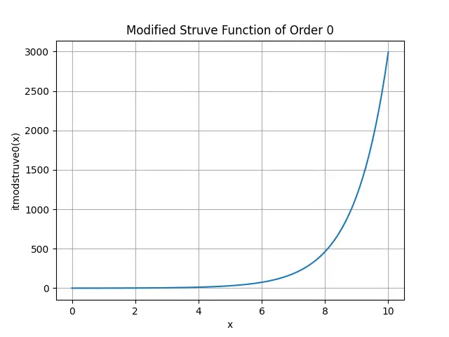
This plots the function across the specified range, effectively visualizing its behavior and characteristics over the interval.

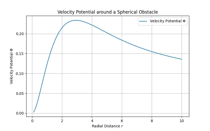
Example 4: Advanced Applications

Imagine we are analyzing the flow around a spherical obstacle in a viscous fluid, and we need to calculate the velocity potential function (ΦΦ) at different points in the fluid. The modified Struve function can appear in solutions to such problems, especially when dealing with spherical coordinates and certain types of potential flow.

Let’s use special.itmodstruve0 to calculate the velocity potential influenced by a specific force distribution. This example is illustrative; the actual application would depend on the specific physical setup and boundary conditions.

import numpy as np
from scipy.special import itmodstruve0
import matplotlib.pyplot as plt

# Define the radial distance from the center of the obstacle
# For illustration, let's consider a range of distances
r = np.linspace(0.1, 10, 400)

# Calculate the modified Struve function for these distances
# Assuming a specific factor in the potential function involves itmodstruve0
potential_factor = itmodstruve0(r)

# For our hypothetical scenario, let's say the total velocity potential
# is influenced by this factor as a part of the solution
# This is a simplified representation
Phi = np.exp(-r) * potential_factor

# Plot the velocity potential as a function of distance
plt.figure(figsize=(8, 5))
plt.plot(r, Phi, label='Velocity Potential $\Phi$')
plt.xlabel('Radial Distance $r$')
plt.ylabel('Velocity Potential $\Phi$')
plt.title('Velocity Potential around a Spherical Obstacle')
plt.legend()
plt.grid(True)
plt.show()

Output:

Explanation:

• r: Represents the radial distance from the center of the spherical obstacle in the fluid.
• potential_factor: Calculated using the modified Struve function, represents part of the potential due to specific force distributions.
• Phi: Represents the velocity potential influenced by the potential_factor. This example uses an exponential decay multiplied by the potential_factor to illustrate the change in potential with distance.
• The plot visualizes how the velocity potential varies with the radial distance from the obstacle.

This example is a simplification and an illustration rather than a precise model of fluid dynamics around a spherical object. In real-world applications, the exact formulation of the potential function and the role of the modified Struve function would depend on the detailed analysis of the forces, boundary conditions, and specific flow characteristics involved in the scenario.

Conclusion

The special.itmodstruve0() function is a potent tool in the SciPy library, showcasing a broad spectrum of applications from basic calculations to advanced scientific computations. Through this tutorial, you’ve seen its versatility and power across various examples. Mastery of such functions can significantly empower your capability in numerical and scientific computing within Python.