SciPy special.yvp() function: A practical guide (4 examples)

Overview

SciPy, the fundamental library for scientific computing in Python, offers a broad spectrum of functions and methods aimed at solving mathematics, science, and engineering problems. Among its extensive collection, the special package stands out, encompassing various special functions beneficial in diverse scientific computations. One such notable function is special.yvp(), designed to calculate derivatives of the Bessel function of the second kind, known as Neumann or Weber functions, Yν(x). Mastering special.yvp() can be immensely useful for individuals working with wave propagation, electrostatics, and numerous other physics applications. This tutorial is a step-by-step guide, illustrated with four progressively complex examples, showcasing the efficacy and versatility of the special.yvp() function in practical applications.

Getting Started with special.yvp()

Before diving into the functional dynamics of special.yvp(), ensure that your Python environment has SciPy installed.

pip install scipy

Once installed, you can start employing the function.

Example 1: Basic Usage

The simplest way to use special.yvp() is to calculate the derivative of the Neumann function for a given order and argument:

import scipy.special as sp
x = 1.0
v = 0
print(sp.yvp(v, x))

Output:

0.7812128213002889

This outputs the value of the first derivative of the Neumann function of order 0 at x=1.0.

Example 2: Varying the Order and Argument

To further understand the utility of special.yvp(), let’s explore how changing the order and the argument affects the output. This will also demonstrate the function’s flexibility:

import scipy.special as sp
for v in range(0, 3):
    for x in range(1, 5):
        print(f'Yv({v})({x}) =', sp.yvp(v, x))

Output:

Yv(0)(1) = 0.7812128213002889
Yv(0)(2) = 0.1070324315409375
Yv(0)(3) = -0.3246744247917997
Yv(0)(4) = -0.39792571055709997
Yv(1)(1) = 0.8694697855159659
Yv(1)(2) = 0.563891888420214
Yv(1)(3) = 0.26862520174885696
Yv(1)(4) = -0.11642216696434
Yv(2)(1) = 2.520152392332221
Yv(2)(2) = 0.5103756726497453
Yv(2)(3) = 0.4316080204484155
Yv(2)(4) = 0.2899739132552924

This script calculates and prints the first derivatives of Neumann functions for orders 0 to 2 and arguments from 1 to 4. The output showcases varying values, reflecting the function’s sensitivity to both parameters.

Example 3: Calculating derivatives at Higher Orders

The special.yvp() function also allows for calculating derivatives of higher orders, enabling in-depth analyses of Bessel functions. This capability is particularly valuable in complex physical and engineering problems.

import scipy.special as sp
x = 2.0
v = 1
derivative_order = 2
print(sp.yvp(v, x, derivative_order))

Output:

-0.20167162055440385

Here, we’ve calculated the second derivative of the Neumann function of order 1 at x=2.0, illustrating special.yvp()’s ability to execute more complex computations.

Example 4: Graphical Representation

Understanding the behavior of Bessel functions and their derivatives can be greatly enhanced through visual representation. This example employs matplotlib to plot the first derivative of Neumann functions over a range of values.

import numpy as np
import scipy.special as sp
import matplotlib.pyplot as plt

x = np.linspace(0.1, 10, 400)
v = 0
y = sp.yvp(v, x)

plt.plot(x, y)
plt.title('Derivative of the Neumann Function')
plt.xlabel('x')
plt.ylabel('yvp(0, x)')
plt.show()

Output:

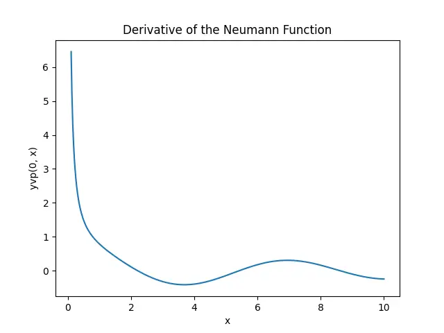
This plot clarifies the oscillatory nature of Neumann function derivatives, providing visual insight into their behavior over a continuous spectrum of values.

Conclusion

The special.yvp() function within SciPy’s special package is a powerful tool for computing derivatives of Neumann (Bessel) functions of the second kind. Through basic usage, variable orders and arguments, higher order derivatives, and visual representation, this tutorial has explored the scope and versatility of special.yvp() in addressing complex scientific problems. The ability to analyze and visualize these functions is instrumental in advancing study and research across various fields of science and engineering.