Introduction
SciPy’s Fast Fourier Transform (FFT) library offers powerful tools for analyzing the frequency components of signals. Within this toolkit, the fft.ifft() function is pivotal for computing the inverse of the Discrete Fourier Transform (DFT), translating frequency-domain data back into the time domain.
Understanding fft.ifft()
The fft.ifft() function is part of the numpy.fft module, which is designed to perform Fourier Transformations efficiently. The inverse FFT operation is crucial for applications where signals need to be analyzed and then reconstructed. This operation effectively undoes the DFT or FFT, converting frequency domain data (complex numbers) back into time-domain signals (real numbers).
To begin, you’ll need to install SciPy if you haven’t already:
pip install scipyExample 1: Basic Inverse FFT
Let’s start with a simple example to see how fft.ifft() function works. Suppose we have a sine wave that we’ve already transformed into the frequency domain. Our goal is to reconstruct the original signal.
import numpy as np
from scipy.fft import ifft

# Frequency domain representation
freq_domain = np.array([0, 4, 0, 0])

# Applying inverse FFT
time_domain = ifft(freq_domain)

print(time_domain)
Output:
[ 1.-0.j 0.+1.j -1.-0.j 0.-1.j]This example demonstrates the basic reconstruction of a sine wave from its frequency-domain representation. The output will be a complex array representing the time-domain signal, showing how fft.ifft() converts between domains.
Example 2: Image Processing
Next, we delve into a more complex application: image processing. Inverse FFT can be used to process and reconstruct images after filtering in the frequency domain.
from scipy.fft import fft2, ifft2
import matplotlib.pyplot as plt
from PIL import Image

# Load and display the original image
image = Image.open('path_to_your_image.jpg').convert('L')
plt.imshow(image, cmap='gray')
plt.title('Original Image')
plt.show()

# Convert image to frequency domain
freq_domain = fft2(image)

# Apply inverse FFT for reconstruction
reconstructed_image = np.abs(ifft2(freq_domain))

# Display the reconstructed image
plt.imshow(reconstructed_image, cmap='gray')
plt.title('Reconstructed Image')
plt.show()
This example highlights the power of fft.ifft() in image reconstruction, showcasing an application beyond simple signal processing.
Example 3: Advanced Signal Manipulation
For our final example, we explore the manipulation of audio signals. We’ll modify the frequency components of an audio file and then reconstruct it using fft.ifft().
The following example requires the package soundfile:
pip install soundfileThe code:
import soundfile as sf
from scipy.fft import fft, ifft

# Load an audio file
audio_signal, samplerate = sf.read('path_to_your_audio_file.wav')

# Convert to frequency domain
freq_domain = fft(audio_signal)

# Perform some manipulation in frequency domain (e.g., filtering noise)
# For illustration, let's just zero out components not in our interest
freq_domain[abs(freq_domain) < 100] = 0

# Reconstruct the audio signal
reconstructed_signal = ifft(freq_domain)

# Save the reconstructed audio
sf.write('reconstructed_audio_file.wav', np.real(reconstructed_signal), samplerate)
This advanced example showcases how fft.ifft() allows for sophisticated manipulation and subsequent reconstruction of audio signals, demonstrating its versatility in signal processing applications.
Conclusion
The fft.ifft() function is a cornerstone in the realm of signal processing, offering a bridge between the frequency and time domains. Its applications range from simple signal reconstruction to complex operations such as image and audio processing. Understanding and utilizing fft.ifft() effectively can unlock new possibilities in various scientific and engineering tasks.
