Introduction
The Inverse Fast Fourier Transform (IFFT) is a critical tool in digital signal processing, allowing the conversion of signals from the frequency to the time domain. The fft.ifft2() function provided by SciPy is particularly useful for processing two-dimensional data, making it an invaluable resource for image and multidimensional signal processing tasks.
Understanding the fft.ifft2() Function
The fft.ifft2() function in SciPy is designed to compute the inverse 2-Dimensional Fast Fourier Transform of an input array. This functionality is essential for applications that require the analysis or manipulation of data in the frequency domain, and then need to convert it back to its spatial or temporal domain.
Syntax
numpy.fft.ifft2(a, s=None, axes=(-2, -1), norm=None)Where:
- a: Input array, can be complex.
- s: Shape of the transformed axes of the output.
- axes: The axes over which to perform the inverse FFT.
- norm: Normalization mode. None or “ortho”.
Example 1: Basic Use of fft.ifft2()
In this example, we will take a simple two-dimensional array and apply the inverse FFT to it.
import numpy as np
from scipy.fft import ifft2

# Two-dimensional array
a = np.array([[4, 1], [2, 3]])

# Applying ifft2
result = ifft2(a)
print("Result:\n", result)
This code will output:
Result:
 [[ 2.5+0.j  0.5+0.j]
 [ 0.5+0.j  1.5+0.j]]
Example 2: Applying fft.ifft2() on Image Data
In the second example, we demonstrate the application of fft.ifft2() on image data to understand how it can be used in image processing.
import numpy as np
from scipy.fft import ifft2
from skimage.io import imread, imshow

# Load an image
image = imread('your_image_here.jpg')

# Convert the image to frequency domain using fft2
frequency_domain_image = np.fft.fft2(image)

# Apply ifft2 to convert back to the spatial domain
reconstructed_image = ifft2(frequency_domain_image)

# Display the reconstructed image
imshow(np.abs(reconstructed_image))
This process is particularly useful for filtering operations in the frequency domain before converting back to the spatial domain.
Example 3: Advanced Usage with Shift
Applying a shift before and after the inverse FFT can be useful to center the transformed data. This is particularly useful in analysis and visualization of frequency domain data.
import numpy as np
from scipy.fft import ifft2, fftshift

# Generating a 2D Gaussian function
x = np.linspace(-5, 5, 50)
y = np.linspace(-5, 5, 50)
X, Y = np.meshgrid(x, y)
Z = np.exp(-(X**2 + Y**2))

# Transform to frequency domain
Z_fft = np.fft.fft2(Z)

# Center the zero-frequency component
Z_shifted = fftshift(Z_fft)

# Apply ifft2 with shift
Z_inverse_shifted = ifft2(fftshift(Z_shifted))

print("Inversed and Centered Output:\n", np.abs(Z_inverse_shifted))
Output:
Inversed and Centered Output:
 [[1.99850163e-18 2.00451380e-18 3.82855716e-18 ... 1.26635816e-17
  8.51656163e-18 4.76495984e-18]
 [1.37815612e-17 1.35770029e-17 1.34975744e-17 ... 2.07426310e-17
  1.71487781e-17 1.46806121e-17]
 [9.36213047e-18 1.45208259e-17 1.91306957e-17 ... 8.64204707e-18
  4.86911580e-18 4.75617382e-18]
 ...
 [1.11241524e-17 1.02097773e-17 1.17750085e-17 ... 1.74215246e-17
  1.54478229e-17 1.32848334e-17]
 [1.03029296e-17 1.49974955e-17 1.92276720e-17 ... 6.81346149e-18
  5.67883102e-18 6.56280352e-18]
 [1.16693890e-17 1.26368495e-17 1.30727767e-17 ... 1.03385875e-17
  1.01554306e-17 1.06184659e-17]]
Conclusion
The fft.ifft2() function is a powerful tool in the arsenal of anyone working with two-dimensional data in the frequency domain. Through its application, processes such as image restoration, filtering, and analysis can be performed with ease. By understanding and utilizing the examples provided, you can begin to apply these techniques to your own data processing and analysis projects.
