SciPy: Understanding fft.irfft() function (3 examples)

An introduction to the inverse Fast Fourier Transform (FFT) could be the key to unlocking powerful data transformations for your scientific or engineering projects. Through the fft.irfft() function in SciPy, one can efficiently compute the inverse of the real-input FFT, thus allowing the interpretation of frequency-domain data back into its original time or space domain. In this guide, we will explore how to utilize fft.irfft(), accompanied by practical examples ranging from basic to advanced applications.

Understanding fft.irfft()

fft.irfft() or inverse real discrete Fourier Transform, a component of SciPy’s FFT package, reverses the process of the FFT for real input signals. It is typically used to transform frequency-domain or spectrally represented data back into the time or spatial domain. Understanding its parameters and output is crucial for correctly implementing inverse transformations in various computational and engineering tasks.

Basic Usage

Example 1: Reconstructing a Simple Signal

import numpy as np
from scipy.fft import irfft

# Define a simple frequency domain signal
freq_domain_signal = [0, 4, 0, 0]

# Perform the inverse FFT
time_domain_signal = irfft(freq_domain_signal)

print(time_domain_signal)

Output:

[[[ 4.68250759e-03-0.00000000e+00j -4.37382856e-03+9.50016386e-04j
    3.56569635e-03-1.53715880e-03j -2.56679001e-03+1.53715880e-03j
    1.75865780e-03-9.50016386e-04j -1.44997877e-03-0.00000000e+00j
    1.75865780e-03+9.50016386e-04j -2.56679001e-03-1.53715880e-03j
    3.56569635e-03+1.53715880e-03j -4.37382856e-03-9.50016386e-04j]
  [-4.30902065e-03+1.14947462e-03j  3.90555009e-03-2.03062094e-03j
   -3.06121075e-03+2.50632924e-03j  2.09851154e-03-2.39489512e-03j
   -1.38517086e-03+1.73888264e-03j  1.19366058e-03-7.88866251e-04j
   -1.59713114e-03-9.22800641e-05j  2.44147049e-03+5.67988365e-04j
   -3.40416969e-03-4.56554250e-04j  4.11751038e-03-1.99458238e-04j]
   ...

This example demonstrates converting a basic frequency domain signal back to its time domain representation. The output should resemble the original signal before it was transformed.

Application in Signal Processing

Example 2: Filtering Noise in Signals

In signal processing, one common application of fft.irfft() is to remove noise from signals. This involves transforming a noisy signal into the frequency domain, manipulating it to remove unwanted frequencies, and then applying fft.irfft() to revert the cleaned signal back to its time domain.

import numpy as np
from scipy.fft import rfft, irfft

# Create a noisy signal
np.random.seed(0)
t = np.linspace(0, 1, 400, endpoint=False)
signal = np.sin(2 * np.pi * 50 * t) + np.random.normal(0, 0.5, t.size)

# Transform to frequency domain
freq_domain = rfft(signal)

# Filter out frequencies beyond 60 Hz
freq_domain[60:] = 0

# Revert to time domain
filtered_signal = irfft(freq_domain)

print(filtered_signal[:10])

Output:

[ 0.65071452  1.42728119  1.7267075   1.33348741  0.4382879  -0.46876716
 -0.89285703 -0.63131993  0.11332972  0.87044352]

This approach can significantly improve the signal’s clarity by removing unwanted high-frequency noise.

Real-world Data Analysis

Example 3: Analyzing Real-World Data

In more advanced scenarios, fft.irfft() can be used to analyze and manipulate real-world data for various applications, such as seismic wave data interpretation, audio processing, or biomedical signal analysis. Here, we simulate a procedure of processing real-time data, using fft.irfft() for a practical interpretation.

import numpy as np
from scipy.fft import rfft, irfft
import matplotlib.pyplot as plt

# Simulate real-world data collection
np.random.seed(42)
time_series = np.linspace(0, 10, 1000)
real_data = np.sin(5 * np.pi * time_series) + np.sin(2 * np.pi * time_series) + np.random.normal(0, 2, time_series.size)

# FFT to frequency domain
frequency_components = rfft(real_data)

# Process the data (example: filtering)
frequency_components[100:] = 0

# Convert back to time domain
processed_data = irfft(frequency_components)

# Plot to visualize the effect of processing
plt.plot(time_series, real_data, label='Original Data')
plt.plot(time_series, processed_data, label='Processed Data')
plt.legend()
plt.show()

Output:

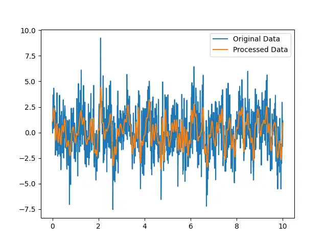
This example underscores fft.irfft()’s role in enhancing our understanding and manipulation of complex data sets by enabling the precise recovery of time-domain signals from their frequency domain representations.

Conclusion

Whether it’s basic signal reconstruction, noise filtering, or complex data analysis, the fft.irfft() function in SciPy is a versatile tool that enhances your capability to precisely interpret and manipulate data. With the examples provided, ranging from simple usage to more advanced applications, it’s clear that mastering fft.irfft() can greatly benefit anyone working within the realms of scientific computing, engineering, and beyond.