Introduction
The fft.irfft2() function in SciPy is an invaluable tool for digital signal processing, particularly in dealing with Fourier transforms. This guide demystifies its workings with practical examples.
Understanding fft.irfft2()
The fft.irfft2() function in SciPy is part of the Fast Fourier Transform (FFT) module, designed to compute the Inverse 2-Dimensional Real-valued FFT. In other words, it takes as input a 2D array of Fourier coefficients, representing the frequency spectrum of a signal, and reconstructs the original signal assuming it was real. This operation is the inverse of the fft.rfft2(), which performs the forward 2D transform from a real-valued signal.
One application of fft.irfft2() is in image processing, where it can reconstruct images from their frequency domain representations, potentially after modifications such as filtering have been applied.
Basic Usage
import numpy as np
from scipy.fft import irfft2

# Creating a 2D array of fourier coefficients
fourier_coeffs = np.zeros((8, 5))
fourier_coeffs[0, 0] = 100 # DC component
fourier_coeffs[1, 1] = 20  # A specific frequency component

# Applying irfft2 to reconstruct the original signal
image = irfft2(fourier_coeffs)

print(image)
Output:
[[2.1875     2.00444174 1.5625     1.12055826 0.9375     1.12055826
  1.5625     2.00444174]
 [2.00444174 1.5625     1.12055826 0.9375     1.12055826 1.5625
  2.00444174 2.1875    ]
 [1.5625     1.12055826 0.9375     1.12055826 1.5625     2.00444174
  2.1875     2.00444174]
  ...
This example demonstrates the most straightforward use of irfft2(), where an array of zeros is manipulated to insert specific Fourier coefficients, and then irfft2() reconstructs the original 2D array (or image). The DC component sets the overall brightness, while other components add details.
Frequency Filtering
import numpy as np
from scipy.fft import irfft2

# Generate a 2D grid of spatial frequencies
freqs = np.fft.fftfreq(16, 0.1)
nyquist_idx = freqs.size // 2
freq_grid = np.zeros((16, nyquist_idx + 1))
freq_grid[2, 3] = 30
freq_grid[3, 2] = 30

# Apply a simple filter to remove high frequencies
filtered_freq_grid = np.copy(freq_grid)
filtered_freq_grid[5:, :] = 0

# Reconstruct the image
filtered_image = irfft2(filtered_freq_grid)
print(filtered_image)
Output:
[[ 4.68750000e-01  2.55419581e-01 -1.65728152e-01 -3.82262417e-01
  -2.34375000e-01  5.08061136e-02  1.65728152e-01  7.60367224e-02
   0.00000000e+00  7.60367224e-02  1.65728152e-01  5.08061136e-02
  -2.34375000e-01 -3.82262417e-01 -1.65728152e-01  2.55419581e-01]
  ...
In this example, a simple spatial frequency grid is created, and specific frequencies are used to generate a pattern. The irfft2() function is then employed to reconstruct the image, demonstrating its potential use in filtering applications where the goal is to manipulate the signal’s frequency domain representation.
Advanced Image Reconstruction
import numpy as np
from scipy.fft import irfft2
import matplotlib.pyplot as plt

# Loading an image as the original signal
original_image = plt.imread('path_to_image.png')
gray_image = np.mean(original_image, axis=-1)  # Convert to grayscale

# Perform the 2D FFT to get frequency components
fourier_image = np.fft.rfft2(gray_image)

# Manipulate the Fourier domain for filtering or other applications
# e.g., setting low frequencies to zero
fourier_image[:2, :2] = 0

# Reconstruct the image from the manipulated Fourier space
reconstructed_image = irfft2(fourier_image)

# Displaying the original and reconstructed images
cmap = 'gray'
plt.figure(figsize=(10, 5))
plt.subplot(1, 2, 1)
plt.imshow(gray_image, cmap=cmap)
plt.title('Original Image')
plt.subplot(1, 2, 2)
plt.imshow(reconstructed_image, cmap=cmap)
plt.title('Reconstructed Image')
plt.show()
This advanced example involves taking a real-world image, converting it to grayscale, applying a 2D FFT to move it into the frequency domain, manipulating the Fourier space, and finally reconstructing the original image. This process illustrates the power of irfft2() in complex signal or image processing tasks, such as noise reduction or resolution improvement.
Conclusion
The fft.irfft2() function in SciPy offers powerful capabilities for signal and image processing through the lens of the Fourier transform. Through the successive complexity of these examples, we’ve seen its versatile applications, from simple reconstructions to sophisticated image manipulations. Such capabilities underscore the importance of mastering FFT operations for professionals in fields ranging from data science to engineering.
