SciPy – Using cluster.hierarchy.cut_tree() function (4 examples)

Overview

The cluster.hierarchy.cut_tree() function in the SciPy library is a powerful tool for cutting hierarchical cluster trees to form flat clusters. Hierarchical clustering is a method of cluster analysis which seeks to build a hierarchy of clusters. In this tutorial, we will explore how to use the cut_tree() function with four different examples, ranging from basic to advanced use cases. You’ll learn not just how to apply this function, but also when and why you might choose to use it in your own data science projects.

Before diving into the examples, it’s essential to have a brief overview of what hierarchical clustering is and how the cut_tree() function fits into it. Hierarchical clustering methods build a multilevel hierarchy of clusters by creating a dendrogram, which is a tree-like diagram that records the sequences of merges or splits.

Example 1: Basic Usage of cut_tree()

What are we doing?

1. Import the necessary libraries and generate hierarchical clusters from some synthetic data.
2. Apply the cut_tree() function to cut the hierarchical tree into flat clusters.

The code:

import numpy as np
from scipy.cluster import hierarchy
from scipy.spatial import distance_matrix

# Generating synthetic data
X = np.array([[1, 2], [3, 4], [4, 5], [6, 7]])

# Computing the distance matrix
D = distance_matrix(X, X)

# Performing hierarchical clustering
Z = hierarchy.linkage(D, 'ward')

# Cutting the hierarchical tree
clusters = hierarchy.cut_tree(Z, n_clusters=2)
print(clusters)

This outputs a set of clusters for our synthetic data:

[[0]
 [0]
 [1]
 [1]]

Example 2: Specifying the Height at Which to Cut the Tree

In this example, we will cut the tree at a specific height, which can be useful for achieving a desired granularity of clustering.

import numpy as np
from scipy.cluster import hierarchy
from scipy.spatial import distance_matrix

# Using the same data as example 1
# Generating synthetic data
X = np.array([[1, 2], [3, 4], [4, 5], [6, 7]])

# Computing the distance matrix
D = distance_matrix(X, X)

# Performing hierarchical clustering
Z = hierarchy.linkage(D, 'ward')

# Cutting the tree at height 3
clusters_at_height = hierarchy.cut_tree(Z, height=3)
print(clusters_at_height)

This yields a different clustering based on the specified tree height:

[[0]
 [1]
 [1]
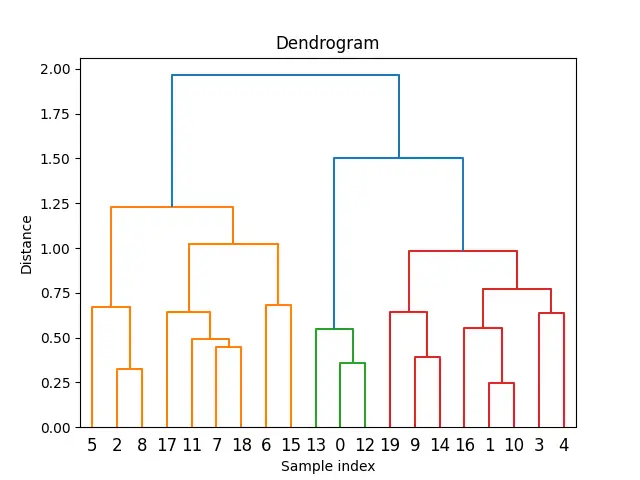
 [2]]

Example 3: Multi-dimensional Data and Plotting Dendrograms

Now, we will work with more complex, multi-dimensional data and illustrate how to plot the dendrogram.

import matplotlib.pyplot as plt
from scipy.cluster import hierarchy
import numpy as np

# Generating multi-dimensional synthetic data
X = np.random.rand(20, 5)

# Hierarchical clustering
Z = hierarchy.linkage(X, method='ward')

# Plotting the dendrogram
plt.figure()
dendrogram = hierarchy.dendrogram(Z)
plt.title('Dendrogram')
plt.xlabel('Sample index')
plt.ylabel('Distance')
plt.show()

# Cutting the tree to form 3 clusters
clusters = hierarchy.cut_tree(Z, n_clusters=3)
print('Clusters:\n', clusters)

The output is a visual dendrogram followed by the cluster assignments:

Clusters:
 [[0]
  [0]
  ...]

Example 4: Advanced Usage – Cutting and Analyzing Clusters

In our final example, we’ll dive deeper into how to analyze clusters obtained by cutting the hierarchical tree in a real-world dataset. We’ll use the Iris dataset to perform hierarchical clustering, cut the tree, and then conduct cluster analysis.

from sklearn.datasets import load_iris
from scipy.cluster import hierarchy
import numpy as np

# Load Iris dataset
iris = load_iris()
X = iris.data

# Hierarchical clustering
Z = hierarchy.linkage(X, 'ward')

# Cutting the tree to form clusters
clusters = hierarchy.cut_tree(Z, n_clusters=3)

# Analyzing clusters
for i in range(3):
    print(f'Cluster {i}:', np.where(clusters == i)[0])

Output:

Cluster 0: [ 0  1  2  3  4  5  6  7  8  9 10 11 12 13 14 15 16 17 18 19 20 21 22 23
 24 25 26 27 28 29 30 31 32 33 34 35 36 37 38 39 40 41 42 43 44 45 46 47
 48 49]
Cluster 1: [ 50  51  52  53  54  55  56  57  58  59  60  61  62  63  64  65  66  67
  68  69  70  71  72  73  74  75  76  78  79  80  81  82  83  84  85  86
  87  88  89  90  91  92  93  94  95  96  97  98  99 101 106 113 114 119
 121 123 126 127 133 134 138 142 146 149]
Cluster 2: [ 77 100 102 103 104 105 107 108 109 110 111 112 115 116 117 118 120 122
 124 125 128 129 130 131 132 135 136 137 139 140 141 143 144 145 147 148]

This will output the indices of the samples belonging to each cluster, exemplifying a way to begin analyzing cluster contents in-depth.

Conclusion

Throughout this tutorial, we’ve explored the cut_tree() function across various contexts, from the simplest applications to more advanced uses with real-world data. Through these examples, it’s clear that cut_tree() is a versatile tool for creating flat clusters from hierarchical structures, facilitating detailed data analysis. As always, the suitability and effectiveness of these techniques depend on the specific requirements of your project and the nature of your data.