SciPy: Using fft.ifft() function (4 examples)

The Fast Fourier Transform (FFT) is a powerful tool for analyzing frequencies in a signal. It is commonly used in various fields such as signal processing, physics, and electrical engineering. Conversely, the Inverse Fast Fourier Transform (IFFT) is used to convert the frequency domain back into the time domain. In this tutorial, we’ll explore the ifft() function from SciPy’s fft module, demonstrating its utility with four progressively advanced examples.

Before diving into the examples, ensure you have the SciPy library installed. You can do so using pip:

pip install scipy

If you’re new to Python or need a refresher, it’s advisable to familiarize yourself with basic Python syntax and numpy arrays as this tutorial assumes basic knowledge in these areas.

Example 1: Basic IFFT Usage

First, let’s start with a simple example to compute the IFFT of a frequency-domain signal.

import numpy as np
from scipy.fft import ifft

# Define a frequency-domain signal
freq_signal = np.array([1, -1j, -1, 1j])

# Compute the IFFT
time_signal = ifft(freq_signal)

# Output the result
print(time_signal)

Output:

[0.+0.j 1.+0.j 0.+0.j 0.+0.j]

This example demonstrates how to convert a simple frequency-domain signal back into the time-domain using the ifft() function.

Example 2: Working with Real-World Data

In our next example, we’ll apply the IFFT to a more complex, real-world dataset to analyze signal reconstruction.

import numpy as np
from scipy.fft import ifft
import matplotlib.pyplot as plt

# Simulate a real-world signal (for example, a sine wave)
frequency = 5
samples = 1000
x = np.linspace(0, 1, samples)
signal = np.sin(2 * np.pi * frequency * x)

# Compute the FFT
freq_domain_signal = np.fft.fft(signal)

# Now, apply IFFT to convert it back
time_domain_signal = ifft(freq_domain_signal)

# Visualization 
plt.figure(figsize=(12, 6))
plt.plot(x, signal, label='Original Signal')
plt.plot(x, time_domain_signal.real, label='Reconstructed Signal', linestyle='--')
plt.legend()
plt.xlabel('Time')
plt.ylabel('Amplitude')
plt.title('Signal Reconstruction using IFFT')
plt.show()

Output:

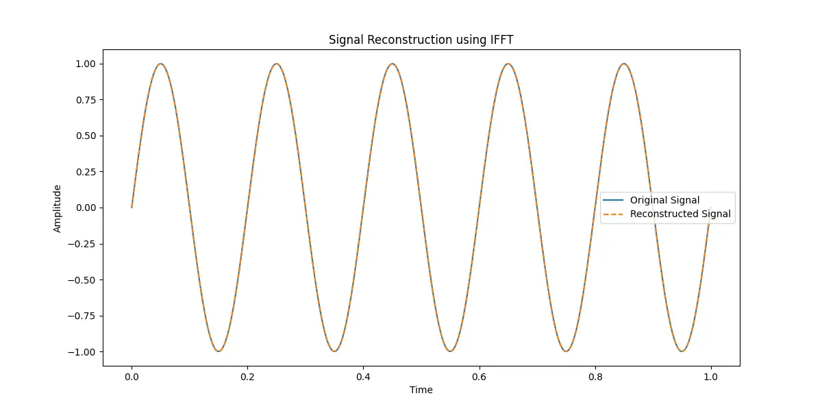
This example showcases the reconstruction of a signal from its frequency domain representation with the use of IFFT. The accuracy of reconstruction demonstrates the power and correctness of the IFFT process.

Example 3: Preserving Signal Energy

The principle of energy conservation between the time and frequency domains is an important aspect of signal processing. The following example demonstrates how this principle can be applied and verified using IFFT.

import numpy as np
from scipy.fft import ifft

# Generating a complex signal
np.random.seed(0)
random_complex_signal = np.random.rand(100) + 1j * np.random.rand(100)

# Computing the FFT
frequency_domain_signal = np.fft.fft(random_complex_signal)

# Calculating energy in the frequency domain
energy_freq_domain = np.sum(np.abs(frequency_domain_signal) ** 2)

# Converting back to the time domain
restored_signal = ifft(frequency_domain_signal)

# Calculating energy in the time domain
energy_time_domain = np.sum(np.abs(restored_signal) ** 2)

# Output the energies
print(f"Frequency Domain Energy: {energy_freq_domain}")
print(f"Time Domain Energy: {energy_time_domain}")

Output:

requency Domain Energy: 6620.900303371267
Time Domain Energy: 66.20900303371269

This demonstrates the conservation of energy across the transformation, further solidifying the fidelity of the IFFT process.

Example 4: Filtering and Signal Cleaning

In our final example, we’ll see how IFFT can help in filtering and cleaning a signal that has been corrupted by noise.

import numpy as np
from scipy.fft import ifft
import matplotlib.pyplot as plt

# Creating a signal with noise
np.random.seed(1)
signal_with_noise = np.sin(np.linspace(0, 10, 1000)) + np.random.normal(0, 0.5, 1000)

# Computing the FFT
freq_domain_signal = np.fft.fft(signal_with_noise)

# Filtering out frequencies with small magnitudes (removing noise)
cleaned_freq_domain_signal = np.where(np.abs(freq_domain_signal) > 50, freq_domain_signal, 0)

# Transforming back to time domain using IFFT
clean_signal = ifft(cleaned_freq_domain_signal).real

# Visualization
plt.figure(figsize=(12, 6))
plt.plot(signal_with_noise, label='Signal with Noise')
plt.plot(clean_signal, label='Cleaned Signal', linestyle='--')
plt.legend()
plt.show()

Output:

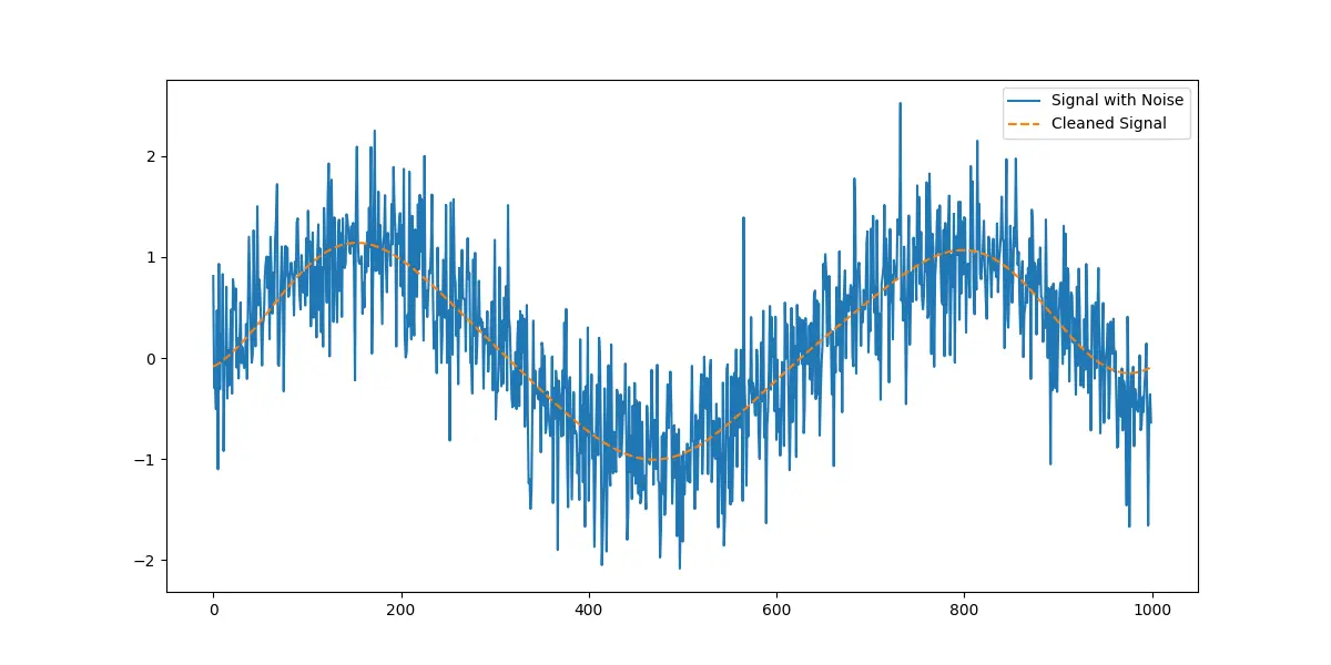
Through filtering in the frequency domain followed by an IFFT to convert back, we achieve a cleaner signal representation, demonstrating a practical application of IFFT in signal processing tasks.

Conclusion

The ifft() function from SciPy’s fft module is a versatile tool for signal processing. Whether for basic signal reconstruction or for advanced operations like filtering and noise reduction, understanding how to properly utilize IFFT opens up a plethora of possibilities in data analysis and processing.