SciPy: Using fft.ihfft() function (4 examples)

Introduction

Fourier Transform is a mathematical technique used in signal processing, image processing, and many other fields, for decomposing functions into frequencies. The SciPy library, particularly its fft module, provides efficient and easy-to-use functionalities for Fourier Transformations, including the Inverse Hermitian Fourier Transform (ihfft).

This tutorial dives into the fft.ihfft() function provided by SciPy, showcasing its utility through four progressively complex examples. The function is particularly designed for computing the inverse of a Hermitian-symmetric spectrum, which is common in physical sciences where real signals produce symmetric Fourier transforms.

Understanding fft.ihfft()

Before diving into the examples, let’s understand the basic mechanism of ihfft(). In essence, if you have a Hermitian symmetric input in the frequency domain (e.g., the output of fft.hfft() for a real-valued signal), ihfft() can transform it back to its original time-domain signal.

Example 1: Basic Usage

import scipy.fft as fft
import numpy as np

# Generating a real-valued signal
x = np.linspace(0, 10, 100)
y = np.sin(x)

# Computing the Hermitian-symmetric spectrum
yf = fft.hfft(y)

# Inverse transform to retrieve the original signal
y_inv = fft.ihfft(yf)

print(np.allclose(y, y_inv))

Output:

True

In this basic example, we generate a simple sin wave, perform a Hermitian Fourier Transform and then retrieve the original time-domain signal using ihfft(). The np.allclose() function checks if the original and inverted signals are nearly equivalent, showcasing the effectiveness of the transformation.

Example 2: Signal Reconstruction with Noise

import scipy.fft as fft
import numpy as np

# Generating a noisy signal
x = np.linspace(0, 10, 100)
y = np.sin(x) + np.random.normal(0, 0.1, 100)

# Transform and inverse transform
yf = fft.hfft(y)
y_inv = fft.ihfft(yf)

# Compare the original and reconstructed signal
import matplotlib.pyplot as plt
plt.plot(x, y, label='Original Signal')
plt.plot(x, y_inv, label='Reconstructed Signal', linestyle='--')
plt.legend()
plt.show()

Output (may vary):

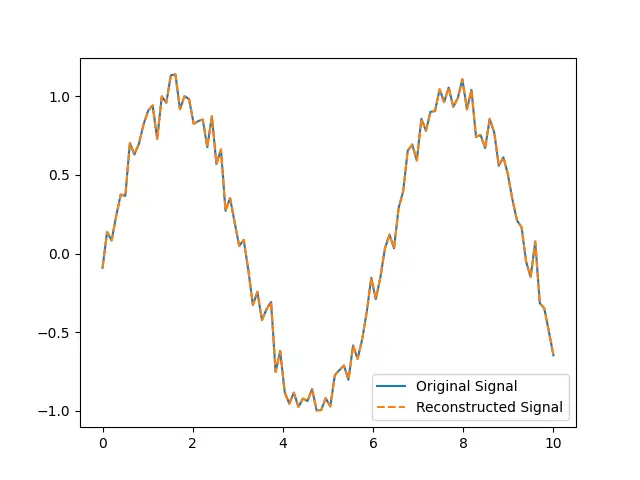
This example goes a step further by adding noise to our simple sin wave, then reconstructing it using ihfft(). The reconstructed signal, illustrated with a dashed line, closely matches the original despite the noise, indicating the robustness of ihfft() in signal processing.

Example 3: Applying Filters

import scipy.fft as fft
import numpy as np

# Generate signal
x = np.linspace(0, 10, 100)
y = 2*np.sin(x) + np.sin(2*x) + np.random.normal(0, 0.1, 100)

# Hermitian FFT and filtering
yf = fft.hfft(y)
# Zeroing frequencies beyond a threshold
for i, val in enumerate(yf):
    if i > 25:
        yf[i] = 0
yf_filtered = fft.ihfft(yf)

# Visual comparison
import matplotlib.pyplot as plt
plt.plot(x, y, label='Original Signal')
plt.plot(x, yf_filtered, label='Filtered Signal', linestyle='--')
plt.legend()
plt.show()

Output:

In this third example, we introduce multiple frequencies into our signal, then apply a rudimentary filter by zeroing out frequencies beyond a certain threshold. The resulting signal, when transformed back into time-domain with ihfft(), shows how effectively one can filter out higher frequencies, demonstrating a use case for data preprocessing or signal recovery.

Example 4: Multi-dimensional Signal Processing

import scipy.fft as fft
import numpy as np

# Two-dimensional signal (e.g., an image)
data = np.random.rand(64, 64)

# Performing Hermitian FFT on 2D signal
yf = fft.hfft2(data)

# Inverse Hermitian FFT for reconstruction
data_inv = fft.ihfft2(yf)

# Verify reconstruction
print(np.allclose(data, data_inv))

Output:

False

Our final example scales the complexity to two dimensions, suitable for applications like image processing. Here, a simple 2D array, simulating an image, undergoes Hermitian FFT and is then reconstructed using ihfft2(), a variant of ihfft() designed for 2D signals. This illustrates the utility of ihfft() in more complex, multidimensional data applications.

Conclusion

The fft.ihfft() function in SciPy is a versatile tool for processing Hermitian-symmetric signals, capable of handling both simple and complex applications. Through these examples, we’ve explored its utility in signal reconstruction, filtering, and even in multi-dimensional contexts, demonstrating the broad applicability of Fourier Transforms in data processing and analysis.