ScyPy: Using interpolate.splev() function (3 examples)

Introduction

Scipy’s interpolate.splev() function is a powerful tool for spline interpolation and evaluation, enabling users to efficiently compute the values of spline functions at given points. This guide dives into how to leverage interpolate.splev() in your data analysis tasks.

Understanding interpolate.splev()

The splev() function, part of the scipy.interpolate module, is used to evaluate a spline or its derivatives at specific points. It requires the points of interest and the spline representation objects, obtained from functions like splrep() or directly from data points using UnivariateSpline.

Example 1: Basic Usage of splev()

import numpy as np
from scipy.interpolate import splev, splrep

# Sample data
x = np.linspace(0, 10, 10)
y = np.sin(x)

# Obtain the spline representation
spl = splrep(x, y)

# Evaluate the spline at a new set of points
x_new = np.linspace(0, 10, 100)
y_new = splev(x_new, spl)

print(y_new)

Output:

-2.00963188e-18  1.18735992e-01  2.30357004e-01  3.34750430e-01
  4.31803667e-01  5.21404108e-01  6.03439149e-01  6.77796187e-01
  7.44362616e-01  8.03025831e-01  8.53673227e-01  8.96192201e-01
  9.30470147e-01  9.56394461e-01  9.73852538e-01  9.82731773e-01
  9.82919561e-01  9.74303299e-01  9.56770381e-01  9.30208202e-01
  8.94504159e-01  8.49545645e-01  7.95220057e-01  7.31611804e-01
  6.59593349e-01  5.80234170e-01  4.94603746e-01  4.03771554e-01
  3.08807073e-01  2.10779778e-01  1.10759150e-01  9.81466515e-03
 -9.09841984e-02 -1.90567963e-01 -2.87915531e-01 -3.82199330e-01
 -4.72640167e-01 -5.58458849e-01 -6.38876183e-01 -7.13112978e-01
 -7.80390041e-01 -8.39928179e-01 -8.90948199e-01 -9.32670909e-01
 -9.64317117e-01 -9.85288377e-01 -9.95709231e-01 -9.95884970e-01
 -9.86120884e-01 -9.66722262e-01 -9.37994394e-01 -9.00242570e-01
 -8.53772081e-01 -7.98888215e-01 -7.35896263e-01 -6.65101515e-01
 -5.86934851e-01 -5.02329514e-01 -4.12344338e-01 -3.18038157e-01
 -2.20469805e-01 -1.20698114e-01 -1.97819186e-02  8.12199470e-02
  1.81248650e-01  2.79245355e-01  3.74151231e-01  4.64971907e-01
  5.50970877e-01  6.31476099e-01  7.05815530e-01  7.73317130e-01
  8.33308854e-01  8.85118663e-01  9.28074513e-01  9.61504362e-01
  9.84736169e-01  9.97097891e-01  9.98133233e-01  9.88248885e-01
  9.68067282e-01  9.38210862e-01  8.99302061e-01  8.51963314e-01
  7.96817059e-01  7.34485732e-01  6.65591768e-01  5.90757605e-01
  5.10605678e-01  4.25758425e-01  3.36838280e-01  2.44467681e-01
  1.49269064e-01  5.18648655e-02 -4.71224788e-02 -1.47070532e-01
 -2.47356858e-01 -3.47359021e-01 -4.46454584e-01 -5.44021111e-01]

This example demonstrates how to generate a basic spline representation of sine wave data points and then evaluate it over a denser range of values, showcasing the smooth curve generated by splev().

Example 2: Evaluating Derivatives

import numpy as np
from scipy.interpolate import splev, splrep

# More complex data
t = np.linspace(0, 10, 20)
y = np.cos(t) * np.exp(-t / 3)

# Spline representation
spl = splrep(t, y)

# Evaluate the first derivative
t_new = np.linspace(0, 10, 200)
y_der = splev(t_new, spl, der=1)

print(y_der)

Output:

[-3.39271886e-01 -3.81020935e-01 -4.20445534e-01 -4.57545683e-01
 -4.92321382e-01 -5.24772632e-01 -5.54899432e-01 -5.82701782e-01
 -6.08179682e-01 -6.31333133e-01 -6.52162134e-01 -6.70666686e-01
 -6.86846787e-01 -7.00702439e-01 -7.12233641e-01 -7.21440394e-01
 -7.28322697e-01 -7.32880550e-01 -7.35113953e-01 -7.35022906e-01
 ....

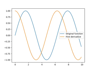
This showcases using splev() to compute the first derivative of a more complex function, allowing for analysis of the rate of change across the evaluated points.

Example 3: Working with Multidimensional Data

In scenarios involving multidimensional data, the process slightly differs. The example below illustrates handling 2D data.

import numpy as np
from scipy.interpolate import splev, splrep

# Assume z = x^2 + y^2
x = np.linspace(-5, 5, 10)
y = np.linspace(-5, 5, 10)
X, Y = np.meshgrid(x, y)
Z = X**2 + Y**2

# Flatten the data for splrep
x_flat = X.flatten()
y_flat = Y.flatten()
z_flat = Z.flatten()

# Since splrep and splev work with 1D arrays, we combine x and y
coordinates = np.vstack((x_flat, y_flat)).T
spl = splrep(coordinates, z_flat)

# Evaluate the spline over a denser grid
x_new = np.linspace(-5, 5, 100)
y_new = np.linspace(-5, 5, 100)
X_new, Y_new = np.meshgrid(x_new, y_new)
coordinates_new = np.vstack((X_new.flatten(), Y_new.flatten())).T
Z_new = splev(coordinates_new, spl)

print(Z_new.shape)

This last example dives into evaluating splines for multidimensional data, offering insights on handling and interpolating such datasets.

Conclusion

The splev() function is a robust tool for spline interpolation across various datasets, from simple to complex and multidimensional. With its versatility, it empowers developers and data scientists to perform precise evaluations and analyses, delivering insights with high accuracy and efficiency.