SciPy – Working with fft.dctn() function (4 examples)

The Discrete Cosine Transform (DCT) is a powerful tool in the realm of signal processing and image compression, found at the heart of standards like JPEG. SciPy, a leading library in scientific computing with Python, provides a comprehensive suite of DCT functions through its fft module. In this tutorial, you’ll learn how to effectively use the fft.dctn() function with four diverse examples, progressing from basic to advanced applications. Understanding dctn() can aid in tasks ranging from data compression to feature extraction in machine learning.

The Fundamentals of fft.dctn()

The fft.dctn() function in SciPy computes the n-dimensional Discrete Cosine Transform (DCT) of an array. This function is part of the scipy.fft module, which provides a wide range of fast Fourier transform routines, including DCT for various types and dimensions.

Syntax:

scipy.fft.dctn(x, type=2, s=None, axes=None, norm=None, overwrite_x=False, workers=None)

Parameters:

• x: array_like. The input array containing the data to be transformed.
• type: {1, 2, 3, 4}, optional. The type of DCT to be performed. The default is 2, which is often used in signal and image processing.
• s: sequence of ints, optional. The shape of the DCT. If given, the first len(s) axes are transformed. If not given, the last len(s) axes are used, or all axes if s is also not specified.
• axes: sequence of ints, optional. Axes over which to compute the DCT. If not specified, the last len(s) axes are used, or all axes if s is not specified.
• norm: {None, ‘ortho’}, optional. Normalization mode. If norm='ortho', the function returns the orthogonal DCT, otherwise, the unnormalized DCT is returned.
• overwrite_x: bool, optional. If True, the contents of x can be destroyed to save memory.
• workers: int, optional. Maximum number of workers to use for parallel computation. The default is None, which means the number of workers is determined by the global setting.

Returns:

• out: ndarray. The n-dimensional DCT of the input array.

Example 1: Basic DCT on a 2D array

Let’s start with the most straightforward application of fft.dctn(): performing a DCT on a two-dimensional array. This example provides a foundation for understanding how the function behaves with multi-dimensional data.

import numpy as np
from scipy.fft import dctn

# 2D array
array = np.array([[1, 2, 3, 4],
                 [5, 6, 7, 8],
                 [9, 10, 11, 12]])

dct_array = dctn(array)
print(dct_array)

This code will output the 2D DCT of the given array. It showcases how dctn() is adept at handling data in arrangements beyond the first dimension.

Output:

[[ 3.12000000e+02 -3.78518644e+01  0.00000000e+00 -2.69004918e+00]
 [-1.10851252e+02  0.00000000e+00  0.00000000e+00  0.00000000e+00]
 [ 1.42108547e-14  0.00000000e+00  0.00000000e+00  0.00000000e+00]]

Example 2: Adjusting DCT Type and Normalization

In this example, we explore adjusting the DCT type and normalization factor, which are crucial for various applications, especially in image processing and compression. The type II DCT is often used in JPEG compression, while the normalization ‘ortho’ ensures energy conservation and can be critical for inverse transformations.

import numpy as np
from scipy.fft import dctn

# Adjusting type and normalization
array = np.array([[1.0, 2.0, 3.0, 4.0],
                 [5.0, 6.0, 7.0, 8.0],
                 [9.0, 10.0, 11.0, 12.0]])

dct_array = dctn(array, type=2, norm='ortho')
print(dct_array)

Output:

[[ 22.5166605   -3.86323973   0.          -0.27455199]
 [-11.3137085    0.           0.           0.        ]
 [  0.           0.           0.           0.        ]]

This output reflects the adjusted DCT behavior, suitable for tasks requiring energy preservation or a particular transform type.

Example 3: Applying DCT on Images

Applying the dctn() to an image is a practical demonstration of its power, especially in the context of image compression. For this example, we’ll load an image using matplotlib, convert it to grayscale, and then apply dctn() to explore its potential in image processing.

import numpy as np
from scipy.fft import dctn
import matplotlib.pyplot as plt
from skimage.color import rgb2gray
from skimage.io import imread

# Load and convert an image to grayscale
image = imread('path/to/image.jpg')
gray_image = rgb2gray(image)

# Applying DCT
image_dct = dctn(gray_image, norm='ortho')

# Displaying the results
plt.imshow(np.log(abs(image_dct)), cmap='gray')
plt.title('DCT of the Image')
plt.colorbar()
plt.show()

This example illustrates how dctn() can help in revealing frequency components, a cornerstone concept in image compression techniques.

Example 4: Advanced Processing with DCT

Building on the previous examples, let’s apply dctn() in a more complex scenario: filtering in the frequency domain and then applying an inverse DCT. This exercise showcases the use of dctn() in signal processing and recovery.

import numpy as np
from scipy.fft import dctn, idctn
import matplotlib.pyplot as plt

# Create a noisy 2D signal
signal = np.random.rand(256, 256)
signal[64:-64, 64:-64] += 4  # Adding a high-value square in the center

# Applying DCT
signal_dct = dctn(signal, norm='ortho')

# Suppressing high-frequency noise
signal_dct[np.abs(signal_dct) < 12] = 0

# Inverse DCT
filtered_signal = idctn(signal_dct, norm='ortho')

plt.imshow(filtered_signal, cmap='gray')
plt.title('Filtered Signal')
plt.show()

Output:

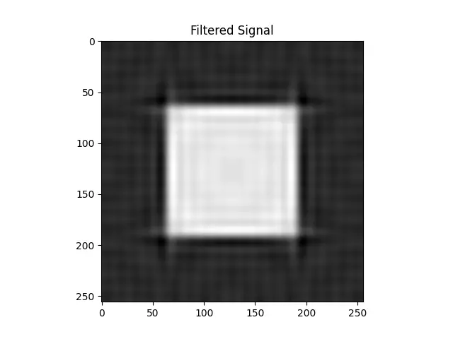
This advanced example demonstrates the utility of dctn() in enhancing and recovering signals, a valuable technique in various applications including signal denoising and restoration.

Conclusion

The fft.dctn() function is a versatile tool for processing multi-dimensional signals. From basic array manipulations to complex image and signal processing, mastering dctn() can unlock new potential in your research or projects, aiding tasks like data compression, feature extraction, and noise reduction.