SciPy: Working with fft.hfftn() function (4 examples)

The fft.hfftn() function in SciPy is a powerful tool for performing N-dimensional half-complex Fast Fourier Transforms (FFTs) on arrays, which can be particularly useful in signal processing, image analysis, and similar fields where interpreting frequency components of multi-dimensional data is necessary. This tutorial aims to provide a comprehensive understanding of the fft.hfftn() function with a progression from basic to advanced usage illustrated through four examples.

Introduction to FFT and SciPy

Before delving into specific examples, it’s important to understand what FFT is and why it’s useful. FFT is an efficient algorithm to compute the Discrete Fourier Transform (DFT) and its inverse. DFT is widely used in engineering, physics, and computer science for analyzing the frequencies contained within a signal. The fft.hfftn() function, specifically, computes the N-dimensional FFT, but only returns half of the result due to the Hermitian symmetry in real inputs, making it computationally efficient for real input data.

Example 1: Basic Usage of fft.hfftn()

import numpy as np
from scipy.fft import hfftn

# Sample array
array = np.array([[1, 2, 3], [4, 5, 6], [7, 8, 9]])

# Applying fft.hfftn()
result = hfftn(array)

# Display the output
print("FFT Result:\n", result)

Output:

FFT Result:
 [[ 60.          -6.           0.          -6.        ]
 [-18.           5.19615242   0.          -5.19615242]
 [-18.          -5.19615242   0.           5.19615242]]

This example demonstrates the straightforward application of fft.hfftn() on a 2-dimensional array. The output reveals the frequency components of the array in a half-complex form, illustrating the basic functionality of the function.

Example 2: Analyzing Frequency Components of an Image

In this example, we will apply the fft.hfftn() to an image to analyze its frequency components. To achieve this, we first need to load an image into a NumPy array.

import matplotlib.pyplot as plt
from scipy.fft import hfftn
from PIL import Image
import numpy as np

# Load the image
image = Image.open('path/to/image.jpg')

# Convert the image to grayscale
image_gray = image.convert('L')

# Convert the grayscale image to a NumPy array
image_array = np.array(image_gray)

# Applying fft.hfftn() to the image
fft_result = hfftn(image_array)

# Displaying the logarithm of the absolute value to observe the frequency spectrum
plt.imshow(np.log(np.abs(fft_result)), cmap='gray')
plt.title('Frequency Components')
plt.colorbar()
plt.show()

This example provides insight into how fft.hfftn() can be used to decipher the frequency components of an image, a valuable technique in image processing for identifying patterns not immediately visible in the spatial domain.

Example 3: The Impact of Windowing

Windowing is a technique used to taper the input signal at its boundaries to reduce the spectrum leakage effect, which is particularly useful when the signal length is not a power of two or when isolating specific frequencies is essential. The following example demonstrates applying a window function before utilizing fft.hfftn().

import numpy as np
from scipy.fft import hfftn
from scipy.signal import windows

# Create a signal
signal = np.random.random((512, 512))

# Apply a Hann window
window = windows.hann(512)
signal_windowed = signal * window[:, None]

# Compute the FFT
fft_result_windowed = hfftn(signal_windowed)

# Display the result
print("With Windowing:\n", fft_result_windowed)

Output (vary):

With Windowing:
 [[ 1.30276038e+05 -3.33529615e+01  4.60250873e+01 ... -1.02253928e+02
   4.60250873e+01 -3.33529615e+01]
 [-6.52121612e+04 -4.36116054e+02 -1.11295984e+01 ...  2.46568513e+02
  -1.07978197e+02  3.58154689e+02]
  ...

Applying a window function before the FFT can significantly improve the analysis’s accuracy by minimizing artifacts. This example illustrates the practical application and benefits of windowing when conducting FFT analysis with fft.hfftn().

Example 4: Multi-Dimensional Signal Processing

The fft.hfftn() is not limited to two-dimensional signals. In this advanced example, we shall see its application in the three-dimensional domain, illustrating its versatility.

import numpy as np
from scipy.fft import hfftn
import matplotlib.pyplot as plt

# Generating a 3D signal
signal_3d = np.random.random((64, 64, 64))

# Conducting FFT
fft_result_3d = hfftn(signal_3d)

# Visualizing a slice of the 3D FFT result
plt.imshow(np.abs(fft_result_3d[:, :, 32]), cmap='gray')
plt.title('3D FFT Slice')
plt.colorbar()
plt.show()

Output (vary):

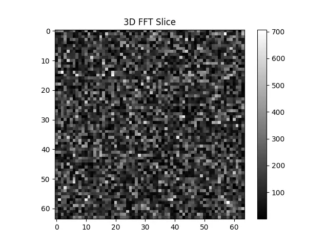
This example moves beyond 2D and showcases the capability of fft.hfftn() to handle 3D data, thus expanding the potential applications of FFT in multi-dimensional signal analysis.

Conclusion

The fft.hfftn() function in SciPy offers a versatile tool for performing N-dimensional half-complex Fast Fourier Transforms. As demonstrated through various examples, its utility spans simple arrays to complex multi-dimensional data, proving invaluable in a plethora of scientific and engineering tasks. Embracing this tool can significantly enhance your data analysis toolkit, whether for basic signal processing or advanced multi-dimensional studies.