The rfftn function in SciPy’s fft module is an indispensable tool for working with Fourier Transforms, especially when dealing with multi-dimensional data. This tutorial will guide you through the basics of using the rfftn() function, moving from elementary examples to more advanced applications. You’ll learn how to apply this function to various types of data and analyze the output effectively.
Introduction to rfftn()
The rfftn() function computes the N-dimensional discrete Fourier Transform for real input. This function is particularly useful for processing real-valued data, offering efficiency advantages over the complex-to-complex Fourier Transform functions for such datasets. Understanding rfftn() is essential for applications in signal processing, image analysis, and scientific computing, where multi-dimensional Fourier Transforms are common.
Getting Started
Before diving into examples, ensure you have Python and SciPy installed on your system. You can install SciPy using pip:
pip install scipyWith the setup out of the way, let’s explore the utilization of rfftn() through comprehensive examples.
Example 1: Basic Application
This first example demonstrates how to perform a Fourier Transform on a simple 2D array using rfftn().
import numpy as np
from scipy.fft import rfftn

# Define a 2D array
array = np.array([[1, 2, 3], [4, 5, 6], [7, 8, 9]])

# Apply rfftn
transformed = rfftn(array)

# Display the result
print(transformed)
Output:
[[ 45. +0.j          -4.5+2.59807621j]
 [-13.5+7.79422863j   0. +0.j        ]
 [-13.5-7.79422863j   0. +0.j        ]]
The output will reflect the frequency domain representation of the input array, illustrating how spatial patterns in the data are encoded into frequencies.
Example 2: Handling Three-dimensional Data
Moving into a more complex scenario, let’s apply the rfftn() function to a 3D array, showcasing its ability to handle volumetric data.
import numpy as np
from scipy.fft import rfftn

# Create a 3D array
array = np.random.rand(4, 4, 4)  # Random 3D array

# Perform the FFT
transformed = rfftn(array)

# Output the result
print(transformed)
Output:
[[[ 3.34670798e+01+0.j          6.14369592e-01+1.83078589j
   -9.03473408e-01+0.j        ]
  [-1.58037458e-01-1.61028282j -8.39769704e-01+2.49658713j
    2.04511811e+00+1.20861459j]
  [-6.27427879e-02+0.j          3.41413248e-03+1.52823942j
    4.51284605e-01+0.j        ]
  [-1.58037458e-01+1.61028282j  2.06234057e+00-2.07756375j
    2.04511811e+00-1.20861459j]]
  ...
This example highlights rfftn()‘s versatility in analyzing multi-dimensional datasets, a crucial capability in fields like medical imaging and 3D modeling.
Example 3: Analyzing Real-world Data
Our third example focuses on applying rfftn() to real-world data, illustrating its practical applications. Here, we use a dataset representing time-series data from multiple sensors.
import numpy as np
from scipy.fft import rfftn
import matplotlib.pyplot as plt

# Assume dataset is loaded into a variable named 'data'
# Apply FFT
transformed = rfftn(data)

# Visualize one dimension of the transformed data
plt.plot(transformed[0])
plt.title('Frequency Spectrum')
plt.xlabel('Frequency')
plt.ylabel('Amplitude')
plt.show()
This visualization of the frequency spectrum allows for the identification of dominant frequencies within the dataset, offering insights into patterns and anomalies.
Example 4: Advanced, Custom Dimensions and Axes
For our final example, we’ll explore how to apply rfftn() to specific dimensions of a dataset, providing refined control over the analysis process.
import numpy as np
from scipy.fft import rfftn

# Higher-dimensional data
array = np.random.rand(6, 6, 6, 6)

# Specify axes for FFT
transformed = rfftn(array, axes=(0, 1, 2))

# Examine the output structure
print(transformed.shape)
Output:
(6, 6, 4, 6)By specifying the axes parameter, we direct rfftn() to perform the Fourier Transform only along the specified dimensions, preserving the original data structure on other axes. This flexibility is invaluable for complex analytical tasks.
Conclusion
This tutorial provided a comprehensive overview of working with the rfftn() function in SciPy, from basic implementations to applying it for the analysis of complex, multi-dimensional datasets. These examples serve as a foundation for exploring the vast potential of Fourier Transforms in real-world applications.
