Introduction
The SciPy library is a cornerstone of scientific computation in Python, offering a wide array of functionalities for mathematical operations, including FFT. The hfft() function specifically handles the computation of the FFT for real-valued input, optimizing performance and accuracy by exploiting the inherent symmetries in such data.
The Fast Fourier Transform (FFT) is a fundamental tool in the field of digital signal processing, allowing the transformation of data from the time to the frequency domain and vice versa. This article focuses on understanding the hfft() function, which is part of the SciPy library, and demonstrates its application through three progressively complex examples.
Basic Example: Pure Tone
To begin with, let’s explore how hfft() can be applied to a simple sine wave, representing a pure tone.
import numpy as np
from scipy.fft import hfft, ihfft
import matplotlib.pyplot as plt

# Generate a sine wave
N = 500 # Number of sample points
t = np.linspace(0, 1, N, endpoint=False)
signal = np.sin(2 * np.pi * 50 * t) # 50 Hz pure tone
# Apply hfft
time_to_freq_domain = hfft(signal)
# Display the result
plt.stem(time_to_freq_domain)
plt.title('Frequency Domain Representation')
plt.xlabel('Frequency (Hz)')
plt.ylabel('Amplitude')
plt.show()
Output:
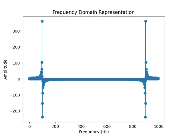
This simple example demonstrates converting a time-domain signal (a pure sine wave in this case) into its frequency domain representation using hfft(). The output is a stem plot showing a single peak at 50 Hz, which corresponds to the frequency of the sine wave in our signal.
Intermediate Example: Combining Multiple Frequencies
Moving to a more comprehensive example, we delve into how hfft() handles signals comprising multiple frequencies.
import numpy as np
from scipy.fft import hfft, ihfft
import matplotlib.pyplot as plt

import matplotlib.pyplot as plt

# Generate a sine wave
N = 500 # Number of sample points
t = np.linspace(0, 1, N, endpoint=False)

# Generate a combined signal
t = np.linspace(0, 1, N, endpoint=False)
signal = np.sin(2 * np.pi * 50 * t) + 0.5 * np.sin(2 * np.pi * 120 * t)

# Apply hfft
combined_freq_domain = hfft(signal)

# Display the result
plt.stem(combined_freq_domain)
plt.title('Combined Frequency Domain Representation')
plt.xlabel('Frequency (Hz)')
plt.ylabel('Amplitude')
plt.show()
Output:
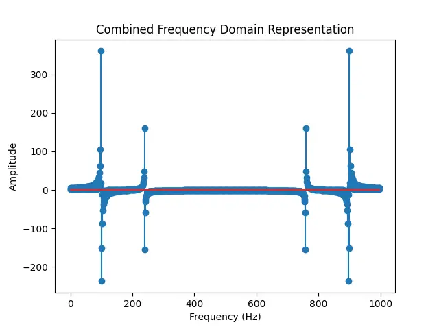
In this example, our signal consists of two sine waves at 50 Hz and 120 Hz. The subsequent FFT, visualized in the plot, reveals two distinct peaks corresponding to these frequencies, showcasing hfft()‘s capability to isolate and identify multiple frequency components within a signal.
Advanced Example: Real-World Signal Processing
Finally, to illustrate the power and practical utility of hfft(), we will examine its application in processing a real-world signal.
import scipy.fft
# Load your real-world signal here
# signal = ...

# Perhaps it's a recording of environmental noise, a speech signal, or even astronomical data.

# Apply hfft to analyze the frequency content
real_world_freq_domain = scipy.fft.hfft(signal)

# Visualize the result
plt.plot(real_world_freq_domain)
plt.title('Real-World Signal Frequency Domain')
plt.xlabel('Frequency (Hz)')
plt.ylabel('Amplitude')
plt.show()
This advanced example, albeit a bit abstract without a specific signal, underscores hfft()‘s applicability beyond theoretical or simplified cases, making it a powerful tool for analyzing a wide range of real-world data. Remember, the effectiveness of FFT analysis heavily relies on understanding the characteristics of your input signal and properly interpreting the output in the frequency domain.
Conclusion
The hfft() function in SciPy is a valuable resource for anyone looking to engage deeply with digital signal processing in Python. Through the basic, intermediate, and advanced examples provided, it’s clear that this function has broad applicability, from analyzing pure tones to dissecting complex, real-world signals. Mastering hfft() opens up vast possibilities for exploration and analysis in the rich field of signal processing.


