Introduction
NumPy is a popular Python library widely used in the field of mathematical modelling for its efficiency in numerical computations and array operations. In this tutorial, we’ll delve into advanced techniques for leveraging NumPy in the context of scientific and engineering problems typically encountered in mathematical modelling.
Getting Started
NumPy, which stands for Numerical Python, is at the heart of scientific computing in Python. It introduces the concept of an n-dimensional array object (ndarray) which is a versatile container of homogenous data, enabling efficient computations on large datasets.
Setting up NumPy is as simple as installing it via pip with the command pip install numpy.
To get started using NumPy, you need to import it into your Python script:
import numpy as npNumPy Basics
Before diving into advanced topics, let’s familiarize ourselves with some basic ndarray operations:
# Creating a basic array
a = np.array([1, 2, 3])
print(a)

# Basic arithmetic operations
b = np.array([1, 1, 1])
print(a + b)
print(a - b)
print(a * b)
print(a / b)
Advanced Indexing and Array Manipulation
Advanced indexing techniques enable complex extraction and manipulation of data from ndarrays. Slice indexing, boolean indexing, and fancy indexing are essential tools for modelling tasks.
# Slice indexing
array2d = np.array([[1, 2, 3], [4, 5, 6], [7, 8, 9]])
slc = array2d[:2, 1:]
print(slc)

# Boolean indexing
bool_idx = array2d > 5
print(array2d[bool_idx])

# Fancy indexing
row_indices = [0, 1, 2]
col_indices = [1, 0, 2]
print(array2d[row_indices, col_indices])
Linear Algebra Operations
NumPy comes with a rich set of functions for linear algebra operations, crucial for solving systems of equations, eigenvalue problems, and other similar tasks.
# Dot Product
v1 = np.array([1, 2, 3])
v2 = np.array([4, 5, 6])
print(np.dot(v1, v2))

# Matrix Multiplication
m1 = np.random.rand(2, 3)
m2 = np.random.rand(3, 2)
print(np.matmul(m1, m2))

# Eigenvalues and Eigenvectors
matrix = np.array([[1, 2], [2, 1]])
vals, vecs = np.linalg.eig(matrix)
print(vals)
print(vecs)
Complex Numbers and Mathematical Functions
Numerical modelling often involves complex numbers and utilizing a broad spectrum of mathematical functions. NumPy provides support for both.
# Dealing with complex numbers
complex_array = np.array([1+2j, 3+4j, 5+6j])
print(np.abs(complex_array))

# Example of mathematical functions
x = np.linspace(-10, 10, 200)
y = np.sin(x)
Randomness in Modelling
Stochastic models necessitate a robust framework for generating random data. NumPy’s random module is ideally suited for this purpose.
# Normal Distribution
normal_data = np.random.normal(loc=0, scale=1, size=(3,3))
print(normal_data)

# Uniform Distribution
uniform_data = np.random.uniform(low=0, high=1, size=(3,3))
print(uniform_data)
Optimizing Computations
Efficient computation is key in numerical modelling, and wisely employing NumPy’s broadcasting, vectorization, and ufunc capabilities can lead to significant performance gains.
# Broadcasting example
scalar = 5
vector = np.array([1, 2, 3])
print(scalar * vector)

# A simple vectorization example
values = np.array([0,
pi/2, np.pi])
sine_values = np.sin(values)
print(sine_values)
Simulating Differential Equations
Many modelling tasks involve solving differential equations. NumPy provides the bedrock upon which solvers like scipy.integrate can build.
# Example: Euler's Method for a simple ODE dy/dx = xy
y0 = 1
h = 0.025
x_end = 2
y_values = [y0]
x_values = np.arange(0, x_end, h)

for x in x_values:
    y = y_values[-1] + h * x_values[-1] * y_values[-1]
    y_values.append(y)

y_values = np.array(y_values)
print(y_values)
Conclusion
NumPy serves as a cornerstone for advanced mathematical modelling in Python. Its array-centric design and powerful toolkit enable practitioners to perform complex computations with ease and efficiency. Whether you’re delving into numerical analysis, stochastic processes, or differential equations, NumPy’s capabilities are essential for robust and performant models.
