The Fast Fourier Transform (FFT) is a powerful computational tool for analyzing the frequency components of time-series data. The fft.fft() function in SciPy is a Python library function that computes the one-dimensional n-point discrete Fourier Transform (DFT) with the efficient Fast Fourier Transform (FFT) algorithm. This tutorial introduces the fft.fft() function and demonstrates how to use it through four different examples, ranging from basic to advanced use cases.
Introduction to FFT and SciPy
Before diving into the examples, let’s understand what FFT and SciPy are. FFT is an algorithm to compute the DFT, which itself converts a signal from its original domain (often time or space) into a representation in the frequency domain. SciPy, on the other hand, is an open-source Python library used for scientific computing and technical computing.
Example 1: Basic FFT
In our first example, we’ll perform a simple FFT on a sine wave to understand how fft.fft() works. Suppose you have a sine wave defined by the function f(t) = sin(2πt), where t is time. Let’s calculate its FFT.
import numpy as np
from scipy.fft import fft
import matplotlib.pyplot as plt

# Sample rate and duration
sr = 1000  # Sample rate in Hz
T = 1  # Duration in seconds

# Time vector
t = np.linspace(0, T, sr, endpoint=False)

# Frequency, in cycles per second, or Hertz
f = 6

# Generate sine wave
y = np.sin(2 * np.pi * f * t)

# Compute the FFT
yf = fft(y)

# Compute the frequencies corresponding to the FFT components
xf = np.fft.fftfreq(len(y), 1 / sr)

# Plotting
plt.plot(xf, np.abs(yf))
plt.title('FFT of a sine wave')
plt.xlabel('Frequency (Hz)')
plt.ylabel('Amplitude')
plt.grid()
plt.show()
Output:
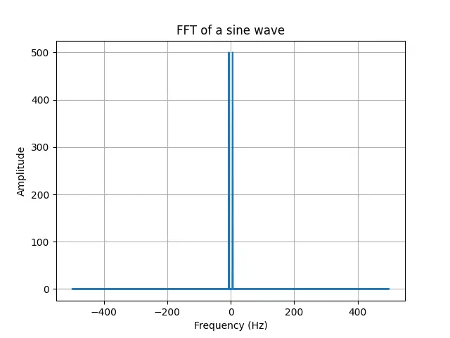
This code generates a sine wave at 6 Hz and computes its FFT. The result is plotted, showing a peak at 6 Hz, which corresponds to the frequency of the sine wave.
Example 2: FFT of a Real-world Signal
Next, let’s analyze a more complex, real-world signal: an audio recording. Here, you’ll see how to use fft.fft() to explore the frequency components of an audio signal.
import numpy as np
from scipy.io import wavfile
from scipy.fft import fft
import matplotlib.pyplot as plt

# Load an audio file
# Replace with your own path
sr, data = wavfile.read('example.wav')

# Compute the FFT of the audio data
yf = fft(data)

# Determine frequency bins
xf = np.fft.fftfreq(len(data), 1 / sr)

# Plot the spectrum
plt.plot(xf, np.abs(yf))
plt.title('FFT of an audio signal')
plt.xlabel('Frequency (Hz)')
plt.ylabel('Amplitude')
plt.show()
This example shows how to load an audio file, compute its FFT, and plot the frequency spectrum. Real-world signals often contain many frequency components, and the FFT allows you to identify and analyze these components.
Example 3: Filtering a Signal Using FFT
FFT can also be used for signal filtering. Here, we’ll apply a simple low-pass filter to an audio signal by manipulating its FFT.
import numpy as np
from scipy.io import wavfile
from scipy.fft import fft, ifft

# Read the audio file
sr, data = wavfile.read('example.wav')

# Compute the FFT of the audio data
yf = fft(data)

# Determine frequency bins (missing in the original snippet)
xf = np.fft.fftfreq(len(data), 1 / sr)

# Apply a low-pass filter
cutoff_frequency = 1000  # Example cutoff frequency
yf[np.abs(xf) > cutoff_frequency] = 0  # Zero out frequencies above the cutoff

# Inverse FFT to get the filtered time-domain signal
filt_signal = np.real(ifft(yf))

# Write the filtered signal to a new WAV file
wavfile.write('filtered_example.wav', sr, filt_signal.astype(np.int16))
This code reads an audio file, applies a FFT, zeros out components above a certain frequency (acting as a low-pass filter), then performs an inverse FFT to convert back to the time domain, and saves the filtered audio. This approach can remove noise or unwanted high-frequency components from signals.
Example 4: Analyzing Multiple Signals Simultaneously
Finally, let’s look at how fft.fft() can be used to analyze multiple signals simultaneously. This is particularly useful in applications like beamforming, where signals from multiple sensors are combined to focus on a particular source.
import numpy as np
from scipy.fft import fft
import matplotlib.pyplot as plt

# Define parameters
sr = 8000  # Sample rate in Hz
T = 1  # Duration in seconds
N = sr * T  # Total number of samples

# Generate a time vector
t = np.linspace(0, T, N, endpoint=False)

# Define example frequencies
freqs = [697, 770, 852, 941]

# Generate individual sine wave signals for each frequency
signals = [np.sin(2 * np.pi * f * t) for f in freqs]

# Combine the individual signals into one composite signal
combined_signal = np.sum(signals, axis=0)

# Perform FFT on the combined signal
yf = fft(combined_signal)

# Compute the frequency bins
xf = np.fft.fftfreq(len(combined_signal), 1 / sr)

# Plot the amplitude spectrum of the FFT
plt.plot(xf, np.abs(yf))
plt.title('FFT of Combined Signals')
plt.xlabel('Frequency (Hz)')
plt.ylabel('Amplitude')
plt.grid()
plt.show()
Output:
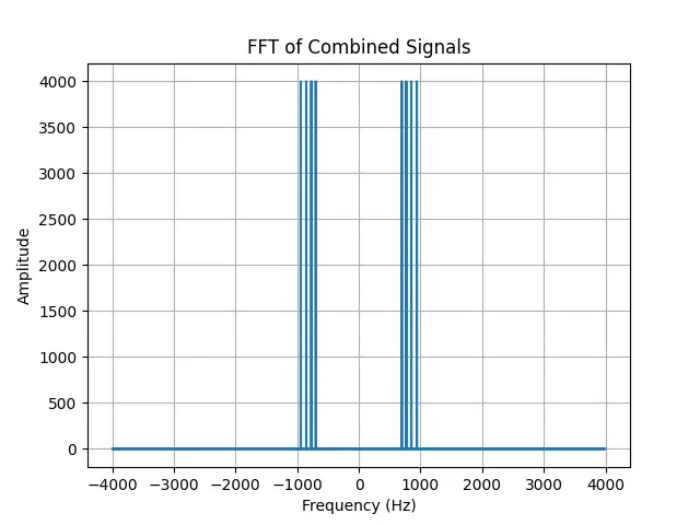
This example demonstrates generating multiple sine waves, combining them, and analyzing the combined signal’s FFT. It showcases the ability of FFT to analyze complex signals composed of multiple frequency components.
Conclusion
The fft.fft() function in SciPy is a versatile tool for frequency analysis in Python. Through these examples, ranging from a simple sine wave to real-world signal processing applications, we’ve explored the breadth of FFT’s capabilities. FFT is not only crucial for understanding signal characteristics but also for advanced signal processing tasks such as filtering and analyzing multiple signals simultaneously.


