How to Use NumPy for Fourier Transform and Frequency Analysis

Introduction

In the realm of digital signal processing, the Fourier Transform is an essential tool. It transforms a signal from its original domain (often time or space) into the domain of frequencies. NumPy, a fundamental package for scientific computing in Python, includes a powerful module named numpy.fft that permits the computation of the Fourier transform and its inverse, alongside various related procedures. This tutorial will guide you through the basics to more advanced utilization of the Fourier Transform in NumPy for frequency analysis.

Getting Started with NumPy Fourier Transform

To begin, ensure NumPy is installed in your Python environment:

pip install numpy

You can import the required module using:

import numpy as np
import numpy.fft as fft

Now let’s apply the Fast Fourier Transform (FFT) to a simple sinusoidal signal:

import matplotlib.pyplot as plt
# Define a time series
N = 600        # Number of data points
T = 1.0 / 800  # Sample spacing
x = np.linspace(0.0, N*T, N)
y = np.sin(50.0 * 2.0*np.pi*x)

# Apply FFT
yf = fft.fft(y)
xf = np.linspace(0.0, 1.0/(2.0*T), N//2)

# Plotting the result
plt.plot(xf, 2.0/N * np.abs(yf[:N//2]))
plt.grid()
plt.show()

Here, we created a sinusoidal signal with a frequency of 50 Hz and applied the FFT to it. The resulting plot displays the magnitude spectrum.

Understanding FFT Outputs

It’s essential to understand what the output from the FFT represents. The Fast Fourier Transform output is a complex array whose magnitude gives the amplitude of the frequency components and the phase angle gives the phase of these components. To analyze the magnitudes of the frequency components, you take the absolute value of the FFT output:

amplitude = np.abs(yf)

Typically, we only need to view the spectrum up to the Nyquist frequency, which is half the sampling rate. That is reflected in us plotting up to N//2.

Signal with Multiple Frequencies

Real signals often have multiple frequency components. For instance:

y = np.sin(50.0 * 2.0*np.pi*x) + 0.5*np.sin(80.0 * 2.0*np.pi*x)
yf = fft.fft(y)
plt.plot(xf, 2.0/N * np.abs(yf[:N//2]))
plt.grid()
plt.show()

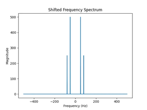
This code plots both the 50 Hz and 80 Hz components in the magnitude spectrum, which are evident in the resulting output.

Windowing

When dealing with finite portions of signals, it’s crucial to apply a window function before the FFT to reduce spectral leakage. Here’s how you can apply a Hanning window to your signal:

window = np.hanning(N)
y_win = y * window
yf_win = fft.fft(y_win)
plt.plot(xf, 2.0/N * np.abs(yf_win[:N//2]))
plt.grid()
plt.show()

The windowing process helps provide a more accurate representation of the signal’s frequency content within the selected segment.

Real Signal Analysis and Understanding Noise

When dealing with actual signals, noise is often present. The FFT can help you understand the noise present in your data. Here’s an example:

# Signal with noise
y_noise = y + 2.5*np.random.randn(N)
yf_noise = fft.fft(y_noise)
plt.plot(xf, 2.0/N * np.abs(yf_noise[:N//2]))
plt.grid()
plt.show()

The plot will include the noise floor created by the random noise added to our signal. In practical applications, strategies such as filtering and signal averaging would be used to handle noise.

Plotting Phase Information

You can also plot the phase information obtained from the FFT:

phase = np.angle(yf)
plt.plot(xf, phase[:N//2])
plt.grid()
plt.show()

This plot demonstrates how the phase of the frequency components is another valuable piece of information that the FFT can provide.

Inverse Fourier Transform

NumPy also allows you to convert the frequency domain back into the original domain—this is known as the inverse Fourier transform (IFFT). Let’s see it in action on our original signal without noise:

yf_ifft = fft.ifft(yf)
plt.plot(x, y)
plt.plot(x, yf_ifft.real)
plt.grid()
plt.show()

The real part of the IFFT’s result closely matches our original y.

Advanced Techniques: Using FFT to Clean a Signal

You can use FFT to remove noise from a signal by zeroing out small Fourier coefficients and then applying an inverse FFT:

# Zero all small coefficients
threshold = 10
yf_clean = yf_noise.copy()
yf_clean[np.abs(yf_noise) < threshold] = 0
# Inverse FFT to get the cleaned signal
y_clean = fft.ifft(yf_clean)

plt.plot(x, y_noise, label='Noisy Signal')
plt.plot(x, y_clean.real, label='Cleaned Signal')
plt.legend()
plt.grid()
plt.show()

Note, this is a simplistic noise reduction technique and more sophisticated methods would be used in real-world applications.

Frequency Analysis of Non-Periodic Signals

The FFT assumes periodic signals. For non-periodic signals, perform your analysis over a section that seems to represent the whole signal well or replicate your non-periodic signal to make it periodic before applying FFT.

Example:

import numpy as np
import matplotlib.pyplot as plt
from scipy.fft import fft

# Generate a non-periodic signal
# For example, a signal that ramps up quickly and then plateaus
t = np.linspace(0, 1, 400, endpoint=False)
signal = np.piecewise(t, [t < 0.2, t >= 0.2], [lambda t: t / 0.2, 1])

# Option 1: Analyze a representative section of the signal
# Select a section that seems to represent the signal well
start, end = 80, 160  # Example indices for a section
signal_section = signal[start:end]
fft_section = fft(signal_section)
frequencies_section = np.fft.fftfreq(len(signal_section), d=(t[1] - t[0]))

# Option 2: Replicate the signal to make it periodic
# Repeat the signal to approximate a periodic signal
replicated_signal = np.tile(signal, 2)  # Repeat the signal twice
fft_replicated = fft(replicated_signal)
frequencies_replicated = np.fft.fftfreq(len(replicated_signal), d=(t[1] - t[0]))

# Plot the original signal and the FFT of both options
plt.figure(figsize=(12, 8))

plt.subplot(3, 1, 1)
plt.plot(t, signal)
plt.title('Original Non-Periodic Signal')

plt.subplot(3, 1, 2)
plt.plot(frequencies_section, np.abs(fft_section))
plt.title('FFT of a Representative Section')

plt.subplot(3, 1, 3)
plt.plot(frequencies_replicated, np.abs(fft_replicated))
plt.title('FFT of Replicated Signal')

plt.tight_layout()
plt.show()

This code snippet demonstrates two approaches for frequency analysis of non-periodic signals:

1. Analyzing a Representative Section: The FFT is applied to a section of the signal that appears to represent its overall behavior.
2. Replicating the Signal: The non-periodic signal is replicated to form a pseudo-periodic signal, and then FFT is applied. This approach can help approximate the frequency content of the original signal.

Conclusion

Total mastery of Fourier transforms is a substantial undertaking, but even at a fundamental level, they are incredibly powerful tools in signal analysis and other fields of science and engineering. With practice and experience, the NumPy FFT module can reveal an abundance of information hidden within signals previously confined to the time domain.