SciPy: Using fft.rfft2() function (4 examples)

In the realm of numerical computing with Python, SciPy stands as a cornerstone library, offering a plethora of functionalities for mathematics, science, and engineering domains. Among its numerous capabilities, the Fourier transform, particularly the fft.rfft2() function, is a powerful tool for analyzing the frequency components of signals and images. This tutorial delves into the use of fft.rfft2(), illuminating its utility through four progressive examples ranging from the basic to the advanced.

What is fft.rfft2()?

The fft.rfft2() function in SciPy performs a two-dimensional Fast Fourier Transform (FFT) on real input. Compared to its counterpart, fft.fft2(), which deals with complex inputs, rfft2() is optimized for real-valued data, offering a more compact output and potentially faster computations. This makes it ideal for tasks such as image processing, where the input data is naturally real.

Example 1: Basic Usage

Let’s start with a simple example that demonstrates the basic functionality of fft.rfft2(). We’ll apply it to a small, artificially created 2D array to understand how it works.

import numpy as np
from scipy.fft import rfft2

# Creating a simple 2D array
data = np.array([[0, 1, 2],
                 [3, 4, 5],
                 [6, 7, 8]])

# Applying fft.rfft2()
fft_result = rfft2(data)
print(fft_result)

Output:

[[ 36. +0.j          4.5+2.59807621j]
 [ -9. +0.j          1.5+0.8660254j ]
 [ -9. +0.j          1.5-0.8660254j ]]

This output represents the frequency components of our input 2D array. The function has condensed the information, reflecting the advantages of using rfft2() for real input.

Example 2: Image Processing

Advancing further, let’s explore how fft.rfft2() can be applied to image processing. We’ll perform a Fourier transform on an image to analyze its frequency components.

from scipy.fft import rfft2
import matplotlib.pyplot as plt
from skimage import data
import numpy as np

# Load an example image from skimage
image = data.camera()

# Apply fft.rfft2()
fft_image = rfft2(image)

# Display the original and the transformed image
fig, axes = plt.subplots(1, 2, figsize=(10, 5))
axes[0].imshow(image, cmap='gray')
axes[0].set_title('Original Image')
axes[1].imshow(np.log(np.abs(fft_image)), cmap='viridis')
axes[1].set_title('Frequency Components')
plt.show()

Output:

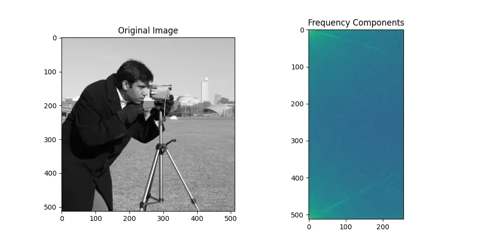
This example showcases how fft.rfft2() can be utilized to uncover the frequency components of an image, providing insights that are critical in various image processing tasks.

Example 3: Applying Filters in Frequency Domain

Moving onto a more intermediate application, we will now explore how to utilize fft.rfft2() for filtering an image in the frequency domain. Filtering in the frequency domain can sometimes be more efficient than doing so in the time/space domain, especially for large images or complex filters.

# Continuing from the previous example

# Construct a simple low-pass filter
filter_size = fft_image.shape
low_pass_filter = np.zeros(filter_size)
low_pass_filter[:50, :50] = 1 # Simple box filter

# Apply the filter
filtered_fft_image = fft_image * low_pass_filter

# Perform the inverse FFT
denoised_image = irfft2(filtered_fft_image)

# Display the results
fig, axes = plt.subplots(1, 2, figsize=(10, 5))
axes[0].imshow(image, cmap='gray')
axes[0].set_title('Original Image')
axes[1].imshow(denoised_image, cmap='gray')
axes[1].set_title('Filtered Image')
plt.show()

Output:

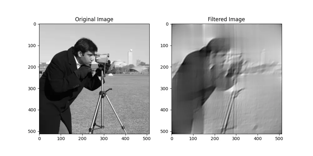
This demonstrates the process of denoising an image by applying a simple low-pass filter in the frequency domain, providing a practical example of fft.rfft2()‘s utility.

Example 4: Advanced Analysis

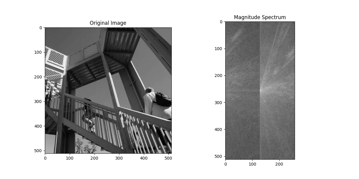
For this advanced example, we’ll perform pattern recognition in the frequency domain by using scipy.fft.rfft2 to analyze an image. This approach is particularly useful for detecting repeating structures within the image, as such patterns manifest as distinct peaks in the frequency domain.

import numpy as np
from scipy.fft import rfft2
import matplotlib.pyplot as plt
from scipy import misc

# Load an example image provided by SciPy
image = misc.ascent()

# The image is already in grayscale, so we can directly use it
image_gray = image

# Apply 2D FFT to the image and shift the zero frequency component to the center
image_fft = rfft2(image_gray)
image_fft_shifted = np.fft.fftshift(image_fft)

# Compute the magnitude spectrum
magnitude_spectrum = np.log(np.abs(image_fft_shifted) + 1)

# Plot the original image and its frequency domain representation
plt.figure(figsize=(12, 6))

plt.subplot(1, 2, 1)
plt.title('Original Image')
plt.imshow(image_gray, cmap='gray')

plt.subplot(1, 2, 2)
plt.title('Magnitude Spectrum')
plt.imshow(magnitude_spectrum, cmap='gray')

plt.show()

By running this code, you’ll see the original ascent image and its frequency domain representation. This demonstrates how repeating patterns and structures within the image translate into peaks in the magnitude spectrum, similar to the original example but without the need for an external image file.

Output:

Conclusion

The fft.rfft2() function in SciPy is a versatile tool for analyzing and manipulating the frequency components of real-valued 2D arrays and images. Through these four examples, ranging from basic to advanced applications, we’ve seen how it can be applied to practical scenarios such as image processing, filtering, and pattern recognition. Mastering fft.rfft2() opens up a world of possibilities for numerical computing in Python.