Introduction
The fft.ifftn() function in SciPy is a powerful tool for computing the n-dimensional inverse discrete Fourier Transform of an array. This article will guide you through its usage with practical examples, ranging from basic to advanced applications.
The Basics of fft.ifftn()
The Fourier Transform is a mathematical technique used to transform a function of time (or space) into a function of frequency. Its inverse, which the fft.ifftn() function calculates, is used to transform back from the frequency domain to the time (or space) domain. The ‘n’ in ifftn indicates that the function is designed to work with n-dimensional data, making it a versatile choice for various scientific and engineering tasks.
# Example 1: Basic Usage
import numpy as np
from scipy.fft import ifftn

# Creating a 2D array
arr = np.array([[1, 2, 3], [4, 5, 6], [7, 8, 9]])

# Applying ifftn
result = ifftn(arr)

print(result)
Output:
[[ 5. -0.j         -0.5-0.28867513j -0.5+0.28867513j]
 [-1.5-0.8660254j   0. +0.j          0. -0.j        ]
 [-1.5+0.8660254j   0. +0.j          0. -0.j        ]]
This example demonstrates the straightforward application of ifftn() to a 2D array. The output will be a 2D array in the complex number form, representing the inverse Fourier Transformed data of the original array.
Advanced Multidimensional Data Handling
As we delve into more complex uses of ifftn, it’s important to understand how it handles multidimensional data. This allows for applications in image processing, 3D modeling, and more.
# Example 2: Image Processing
import matplotlib.pyplot as plt
from scipy.fft import ifftn
import numpy as np

# Simulating a frequency domain representation of an image
frequency_domain = np.random.rand(256, 256)

# Applying ifftn to simulate obtaining the original image
image = ifftn(frequency_domain)

# Displaying the 'image'
plt.imshow(np.abs(image), cmap='gray')
plt.title('Simulated Image')
plt.show()
Output (might vary):
In this example, we simulate the inverse transformation of an image’s frequency domain representation back to its spatial domain equivalent. This highlights ifftn‘s capability in image reconstruction, a vital function in various imaging technologies.
Applying Masking and Filters
Another advanced use of ifftn is its application in data analysis, particularly through the application of masks or filters before performing the inverse transformation. This technique is useful in signal and image processing for isolating or eliminating certain frequencies.
# Example 3: Filtering
import numpy as np
from scipy.fft import ifftn

# Creating a 3D data set representing a signal
signal = np.random.rand(10, 10, 10)

# Creating a mask to apply a simple filter
mask = np.zeros((10, 10, 10))
mask[4:6, 4:6, 4:6] = 1

# Applying mask
filtered_freq_domain = signal * mask

# Processing with ifftn
processed_signal = ifftn(filtered_freq_domain)

print(processed_signal)
Output (very long):
[[[ 5.57704909e-03-0.00000000e+00j -5.12471116e-03+1.39215301e-03j
    3.94047508e-03-2.25255088e-03j -2.47667878e-03+2.25255088e-03j
    1.29244270e-03-1.39215301e-03j -8.40104767e-04-0.00000000e+00j
    1.29244270e-03+1.39215301e-03j -2.47667878e-03-2.25255088e-03j
    3.94047508e-03+2.25255088e-03j -5.12471116e-03-1.39215301e-03j]
    ....
In this more complex example, we apply a straightforward filter to a 3D data set before inverse transforming it. The mask effectively isolates a specific frequency band, allowing for focused analysis or reconstruction of the signal.
Conclusion
The fft.ifftn() function is a cornerstone in the computational analysis of signals and images across multiple dimensions. Through the examples provided, we’ve seen its basic operation, handling of multidimensional data, and its advanced applications in filtering. Whether you’re working in engineering, physics, or digital art, understanding how to use fft.ifftn() can significantly expand your analytical toolkit.
