In this tutorial, we delve into the SciPy library’s interpolate.splder() function, a powerful tool for differentiating splines in Python. Understanding and applying this function correctly can provide a significant advantage in data analysis, physics simulations, and more. We’ll start with the basics and gradually move to more advanced examples.
Prerequisites:
- Basic knowledge of Python programming.
- Familiarity with numerical computing in Python.
- An installed version of SciPy in your working environment.
What does interpolate.splder() Do?
The interpolate.splder() function in SciPy is used to compute the derivative of a spline representation. Essentially, if you’ve created a spline representation of your data—for instance, using interpolate.splrep()—you can then apply splder() to obtain its derivative at various points or intervals.
Example 1: Creating a Spline and Computing Its First Derivative
from scipy import interpolate
import numpy as np
import matplotlib.pyplot as plt

# Sample data
x = np.arange(0, 10, 0.1)
y = np.sin(x)

# Create a spline representation
tck = interpolate.splrep(x, y, s=0)

# Derive the first derivative
first_derivative = interpolate.splder(tck, n=1)

# Plot
plt.figure()
plt.plot(x, y, label='Original function')
plt.plot(x, interpolate.splev(x, first_derivative), label='First derivative')
plt.legend()
plt.show()
Output:
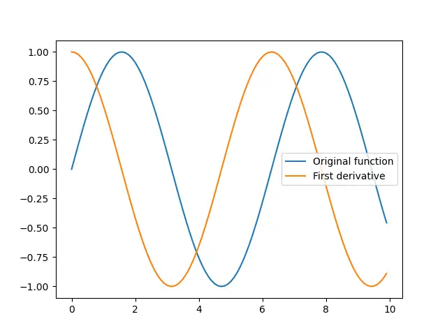
This example demonstrates the primary use case of interpolate.splder(): computing and plotting the first derivative of a given function.
Example 2: Extracting Higher Order Derivatives
from scipy import interpolate
import numpy as np
import matplotlib.pyplot as plt

# Continuing from the previous example, let's extract the second derivative
second_derivative = interpolate.splder(tck, n=2)

# Plot
plt.figure()
plt.plot(x, interpolate.splev(x, second_derivative), label='Second derivative')
plt.legend()
plt.show()
Output:
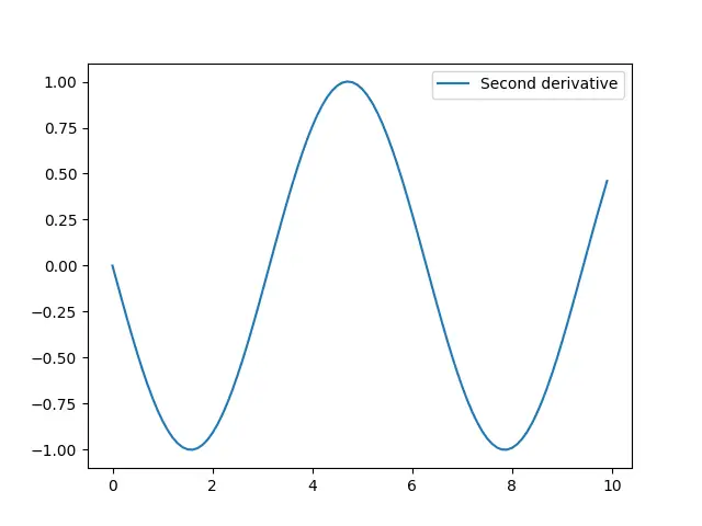
This example shows how to compute and visualize higher-order derivatives using the same spline representation. By setting the n parameter, you can specify which derivative to calculate.
Example 3: Working with Complex Splines
As we delve into more complex examples, consider how splder() can be utilized in situations with oscillatory behavior, multisdimensinal data, or retrospective interpolation adjustments.
from scipy import interpolate
import numpy as np
import matplotlib.pyplot as plt

# Create a complex spline representation
x = np.linspace(0, 10, 200)
y = np.exp(-x**2) + np.cos(x)
tck = interpolate.splrep(x, y, s=0)

# Derive the first derivative for complex function
first_derivative_complex = interpolate.splder(tck, n=1)

# Plot
plt.figure()
plt.plot(x, y, 'b-', label='Original function')
plt.plot(x, interpolate.splev(x, first_derivative_complex), 'r-', label='First derivative')
plt.legend()
plt.show()
This example showcases interpolate.splder() applied to a complex function’s derivative. By adjusting the original function, you can observe how the derivative adapts to more complex, real-world data.
Error Handling and Edge Cases
Understanding error handling and edge cases in splder() is essential for robust implementation. For instance, attempting to take a derivative higher than the spline’s degree results in an error. Therefore, ensuring compatibility between the spline’s order and the desired derivative’s order is crucial.
Conclusion
The interpolate.splder() function in SciPy offers a versatile and efficient means for differentiating spline representations of data. From basic first derivatives to more intricate applications and edge case handling, our journey through these examples illuminates the function’s breadth of use and adaptability in a range of scenarios. With these tools, your analytical and computational skillset is now even more powerful.