NumPy: Getting samples from a noncentral chi-square distribution (5 examples)

Overview

The NumPy library is an indispensable tool for numerical computing in Python, providing support for large, multi-dimensional arrays and matrices, along with a collection of mathematical functions to operate on these arrays. One of the specialized functionalities that NumPy offers is the ability to generate random samples from various statistical distributions, including the noncentral chi-square distribution. This tutorial will walk you through how to draw samples from a noncentral chi-square distribution using NumPy, progressively covering from basic to more advanced examples.

Example 1: Basic Sampling

To start, let’s learn how to draw a simple sample from a noncentral chi-square distribution. In NumPy, this can be accomplished using the np.random.noncentral_chisquare function. Let’s generate 10 random samples from a noncentral chi-square distribution with 3 degrees of freedom and a noncentrality parameter of 2.0:

import numpy as np

# Define parameters
degrees_of_freedom = 3
noncentrality = 2.0

# Generate samples
samples = np.random.noncentral_chisquare(degrees_of_freedom, noncentrality, size=10)

print(samples)

The output will display an array of 10 numbers, each representing a sample from the specified distribution.

Here’s a possible output:

[ 1.61003007  8.4569624   3.54728345  3.82562967 17.46616173  8.14668565
  2.72886743 15.23239307  0.7108787   6.10076469]

Example 2: Visualizing the Distribution

After generating the samples, you might want to visualize the distribution to better understand its shape and spread. Plotting histograms of the sampled data is a straightforward approach:

import matplotlib.pyplot as plt
import numpy as np

# Define parameters
degrees_of_freedom = 3
noncentrality = 2.0

# Generate samples
samples = np.random.noncentral_chisquare(
    degrees_of_freedom, noncentrality, size=10)


# Plot a histogram
plt.hist(samples, bins=10, density=True, alpha=0.6, color='g')
plt.show()

Output (vary):

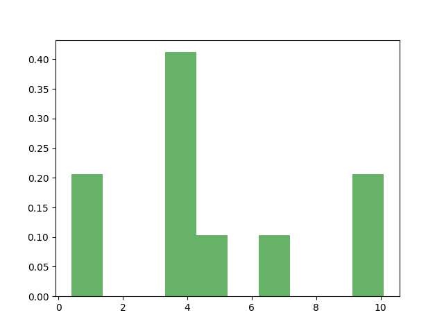
This graph provides a visual representation of how the samples are distributed, which might help in understanding the theoretical properties of the noncentral chi-square distribution.

Example 3: Sample Size Impact

Next, let’s examine the effect of changing the sample size. The size of your sample can significantly impact the approximation to the theoretical distribution. This example will compare smaller and larger sample sizes:

import matplotlib.pyplot as plt
import numpy as np

# Define parameters
degrees_of_freedom = 3
noncentrality = 2.0

# Larger sample size
large_samples = np.random.noncentral_chisquare(
    degrees_of_freedom, noncentrality, size=1000)

plt.hist(large_samples, bins=30, density=True, alpha=0.6, color='r')
plt.show()

Output (vary, due to the randomness):

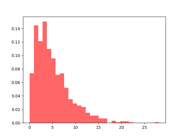
With a larger sample size, the histogram appears smoother and closer to the theoretical distribution. This is a clear indication of the law of large numbers in action.

Example 4: Comparing Different Noncentrality Parameters

Now we will examine how different noncentrality parameters affect the distribution. By generating samples with varying noncentrality parameters but keeping the degrees of freedom constant, we can observe shifts and shape changes in the distribution:

import matplotlib.pyplot as plt
import numpy as np

# Define parameters
degrees_of_freedom = 3
noncentrality = 2.0

# Samples with different noncentrality parameters
param1_samples = np.random.noncentral_chisquare(
    degrees_of_freedom, 1.0, size=1000)
param2_samples = np.random.noncentral_chisquare(
    degrees_of_freedom, 5.0, size=1000)

plt.hist(param1_samples, bins=30, density=True, alpha=0.6, color='blue')
plt.hist(param2_samples, bins=30, density=True, alpha=0.6, color='orange')
plt.show()

Output (vary):

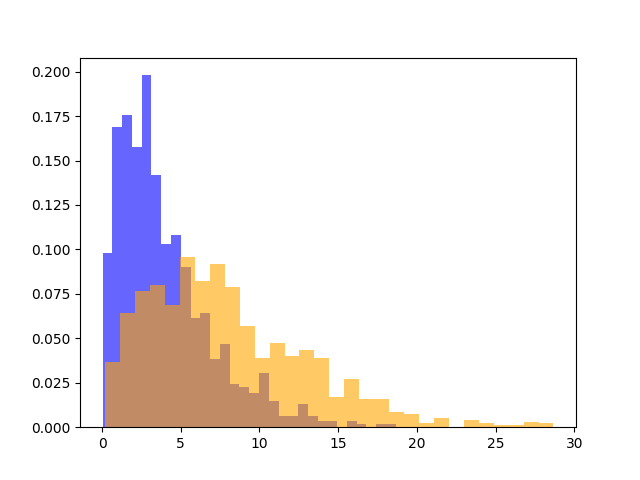
This comparison prominently highlights how the noncentrality parameter influences the distribution’s center and spread. Understanding this relation is critical for various statistical analyses and simulations.

Example 5: Replicability with Seed

Lastly, for scientific reproducibility, it’s important to produce the same set of samples across different runs of the experiment or analysis. NumPy offers a simple way to achieve this using seeds:

import matplotlib.pyplot as plt
import numpy as np

# Setting the seed for reproducibility
np.random.seed(42)

# Define parameters
degrees_of_freedom = 3
noncentrality = 2.0


# Generating samples with a fixed seed
replicable_samples = np.random.noncentral_chisquare(
    degrees_of_freedom, noncentrality, size=10)

print(replicable_samples)

Output:

[1.02994169 3.34288278 2.98678954 8.34181011 0.73604655 1.19562164
 2.16151531 6.27969991 2.86526808 1.36387871]

By setting a seed, we ensure that anyone running this code snippet will get the exact same set of samples, which is essential for verifiable scientific experiments and peer reviews.

Conclusion

Drawing samples from a noncentral chi-square distribution in NumPy is a versatile technique that provides valuable insights into statistical properties and hypotheses testing. Starting with basic sampling and moving towards more sophisticated explorations, including visualizations and the effect of various parameters, enhances your understanding of the noncentral chi-square distribution. Ensuring the replicability of your experiments using seeds is crucial for maintainable and credible scientific computing.