SciPy cluster.hierarchy.cophenet() function (4 examples)

Overview

In this tutorial, we’ll dive deep into the cophenet() function provided by SciPy’s cluster.hierarchy module. This function is a vital tool for hierarchical clustering analysis, as it measures the cophenetic correlation coefficient of a hierarchical clustering. The cophenetic correlation coefficient is a measure of how faithfully a dendrogram preserves the pairwise distances between the original unmodeled data points. A higher coefficient indicates a dendrogram that more accurately represents the original data.

We’ll explore the cophenet() function through four progressively more complex examples, starting from the basics of performing hierarchical clustering and calculating the cophenetic correlation coefficient, to utilizing it in dataset analysis with visualizations. Let’s get started.

Example 1: Basic Usage of cophenet()

from scipy.cluster.hierarchy import linkage, cophenet
from scipy.spatial.distance import pdist
import numpy as np

# Sample data
X = np.array([[1, 2], [2, 3], [3, 2], [4, 4]])

# Perform hierarchical clustering
Z = linkage(X, 'ward')

# Calculate the cophenetic correlation coefficient
c, coph_dists = cophenet(Z, pdist(X))
print("Cophenetic correlation coefficient:", c)

Output:

Cophenetic correlation coefficient: 0.7489751329583314

This first example demonstrates the simplicity of using cophenet() to assess the quality of hierarchical clustering. The function takes two arguments: the linkage matrix Z generated by linkage(), and the distances between the original data points, calculated here by pdist(). The output is the cophenetic correlation coefficient, achieving a quantitative measure of the dendrogram’s accuracy.

Example 2: Visualizing the Dendrogram and Calculating the Cophenetic Correlation

from scipy.cluster.hierarchy import linkage, cophenet
from scipy.spatial.distance import pdist
import numpy as np

from matplotlib import pyplot as plt
from scipy.cluster.hierarchy import dendrogram

# Re-using the previous setup for hierarchical clustering
# Sample data
X = np.array([[1, 2], [2, 3], [3, 2], [4, 4]])

# Perform hierarchical clustering
Z = linkage(X, 'ward')

# Plot dendrogram
plt.figure(figsize=(10, 7))
plt.title('Hierarchical Clustering Dendrogram')
dendrogram(Z)
plt.show()

Output:

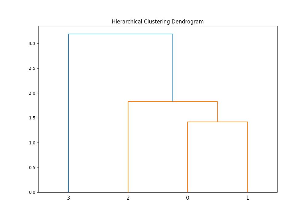
After performing the clustering, visualizing the results can provide further insight. By plotting the dendrogram, we gain visual confirmation of the clustering quality, which complements the quantitative measure provided by the cophenetic correlation coefficient. This example reinforces the importance of visual analysis in data science and statistics.

Example 3: Advanced Analysis Using Cophenet for Different Linkage Methods

import numpy as np
from scipy.cluster.hierarchy import linkage, cophenet
from scipy.spatial.distance import pdist
from scipy.cluster.hierarchy import complete, average, single


# Generate more complex data
X = np.random.random((20, 2))

# Perform hierarchical clustering using different methods
Z_ward = linkage(X, 'ward')
Z_complete = complete(X)
Z_average = average(X)
Z_single = single(X)

# Calculate the cophenetic correlation coefficient for each linkage method
ward_c, _ = cophenet(Z_ward, pdist(X))
complete_c, _ = cophenet(Z_complete, pdist(X))
average_c, _ = cophenet(Z_average, pdist(X))
single_c, _ = cophenet(Z_single, pdist(X))

# Output the results
print("Ward linkage cophenetic correlation:", ward_c)
print("Complete linkage cophenetic correlation:", complete_c)
print("Average linkage cophenetic correlation:", average_c)
print("Single linkage cophenetic correlation:", single_c)

Output (vary, due to the randomness):

Ward linkage cophenetic correlation: 0.7448419614411551
Complete linkage cophenetic correlation: 0.7214064745839055
Average linkage cophenetic correlation: 0.7742684039844714
Single linkage cophenetic correlation: 0.7521312528673432

This third example takes our understanding further by comparing the cophenetic correlation coefficients across different linkage methods. Hierarchical clustering can be performed using various strategies, each impacting the resulting dendrogram’s structure. By calculating and comparing these coefficients, we discern which method best preserves the inter-point distances of the original dataset, offering valuable insights for data analysis projects.

Example 4: Integrating cophenet with Real-World Data

For an advanced example involving scipy.cluster.hierarchy.cophenet() with real-world data, we’ll perform hierarchical clustering on a dataset and evaluate the cophenetic correlation coefficient to measure how faithfully the dendrogram preserves the pairwise distances between the original unmodeled data points. We will use the Iris dataset for this purpose, a popular dataset in machine learning and statistics that includes measurements of 150 iris flowers from three different species.

Steps:

1. Load the Iris dataset.
2. Perform hierarchical clustering.
3. Compute the cophenetic correlation coefficient.
4. Plot the dendrogram.

The code:

import numpy as np
import matplotlib.pyplot as plt
from scipy.cluster.hierarchy import dendrogram, linkage, cophenet
from scipy.spatial.distance import pdist
from sklearn.datasets import load_iris

# Step 1: Load the Iris dataset
iris = load_iris()
X = iris.data

# Step 2: Perform hierarchical clustering
Z = linkage(X, 'ward')

# Step 3: Compute the cophenetic correlation coefficient
c, coph_dists = cophenet(Z, pdist(X))
print(f"Cophenetic Correlation Coefficient: {c}")

# Step 4: Plot the dendrogram
plt.figure(figsize=(10, 8))
dendrogram(Z, labels=iris.target, color_threshold=0)
plt.title("Hierarchical Clustering Dendrogram (Iris dataset)")
plt.xlabel("Sample index")
plt.ylabel("Distance")
plt.show()

You’ll see this diagram:

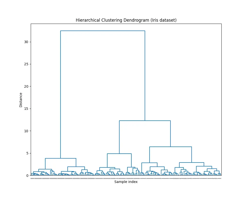
And this output:

Cophenetic Correlation Coefficient: 0.8728283153305715

Conclusion

The cophenet() function is a powerful tool for evaluating the reliability of hierarchical clustering by measuring the cophenetic correlation coefficient. This tutorial showcased its utility from basic to advanced examples, enhancing our understanding of its role in data analysis. Whether for academic research or industrial applications, integrating cophenet into your clustering analysis workflow can dramatically improve insights and decision-making.