SciPy fft.dst() function (4 examples)

In this tutorial, we’ll dive deep into understanding the Discrete Sine Transform (DST) function available in the SciPy library, specifically fft.dst(). DST is an essential tool in signal processing, often used for separating different frequencies in a wave, which makes it vital for audio signal analysis, image processing, and solving partial differential equations. We’ll explore this function with four progressively complex examples.

What is DST?

Before we jump into the coding examples, let’s get a brief overview of what Discrete Sine Transform is. The Discrete Sine Transform (DST) transforms a list of n real numbers into another list of real numbers. Essentially, it transforms spatial domain data into frequency domain data. It’s particularly useful in scenarios where boundary conditions are specified using sine functions.

SciPy fft.dst() implementation provides an accessible way to compute DST. Different types of DSTs (I, II, III, and IV) can be computed using this function by specifying the type parameter.

Example 1: Basic Usage of DST

Let’s start with a simple example, performing a Type II DST on a basic set of real numbers.

from scipy.fft import dst

# Our simple data set
x = [0, 1, 2, 3, 4]

# Performing Type II DST
y = dst(x, type=2)

print(y)

Output:

[ 10. -4.3524 0. -1.3811 0. ]

This output represents the transformed frequency domain data of our input array x. Notice how the DST has separated the component frequencies.

Example 2: DST on Image Data

Now, let’s apply DST to process image data. We’ll use a grayscale image, transform it using DST to manipulate it, and then revert back to the spatial domain to observe the manipulation.

import numpy as np
from scipy.fft import dst, idst
from matplotlib import pyplot as plt
from skimage import data, color

# Load a sample image and convert to grayscale
image = color.rgb2gray(data.astronaut())

# Applying DST
trans_image = dst(dst(image.T, type=2).T, type=2)

# Applying inverse DST
dst_back = idst(idst(trans_image.T, type=2).T, type=2)

plt.figure(figsize=(10, 5))
plt.subplot(121)
plt.imshow(image, cmap='gray')
plt.title('Original Image')
plt.subplot(122)
plt.imshow(dst_back, cmap='gray')
plt.title('After DST and Inverse DST')
plt.show()

Output:

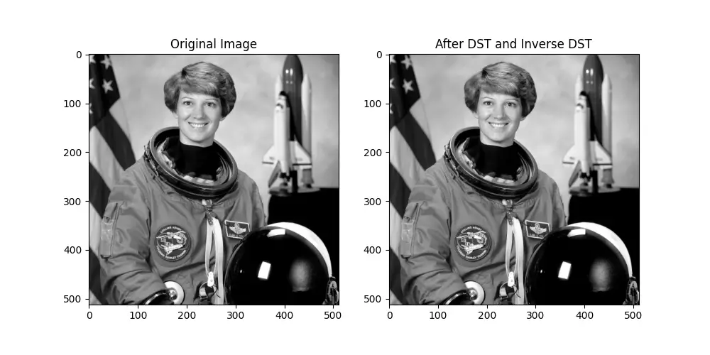
This code loads an astronaut’s image, applies DST to it, and then converts it back using the inverse DST. The output should show two images side by side where changes might be subtle but indicate the effect of the transformation.

Example 3: Higher-Dimensional Data

DST is not limited to one-dimensional data; it can also be applied to multidimensional data. Let’s see how to apply DST on a two-dimensional Numpy array representing a matrix.

import numpy as np
from scipy.fft import dst

# 2D array
matrix = np.array([[0, 1, 2], [3, 4, 5], [6, 7, 8]])

# Applying DST on each axis
dst_matrix = dst(dst(matrix, axis=0, type=2), axis=1, type=2)

print(dst_matrix)

Output:

[[ 64.         -13.85640646  32.        ]
 [-41.56921938   0.         -20.78460969]
 [ 32.          -6.92820323  16. 

This example illustrates the flexibility of fft.dst() in dealing with 2D arrays, which can be especially useful in image processing and numerical simulations.

Example 4: Advanced Use: Solving Differential Equations

One valuable application of DST is in solving differential equations. Here, we’ll demonstrate solving a boundary value problem using DST.

from scipy.fft import dst, idst
import numpy as np
import matplotlib.pyplot as plt

# Define the grid and differential equation parameters
N = 100
x = np.linspace(0, np.pi, N)
h = x[1] - x[0]
f = np.sin(x)

# DST of the function f using type=2
F = dst(f, type=2, norm='ortho')

# Solve the differential equation in the frequency domain
k = np.arange(1, N+1)  # Adjusted to match the output of dst
L = np.tan((k - 1) * h / 2)  # k - 1 to account for zero-based indexing in Python
F /= (L**2 + 1)

# Perform inverse DST using type=2
g = idst(F, type=2, norm='ortho')

# Plotting the results
plt.plot(x, g, label='g(x)')
plt.xlabel('x')
plt.ylabel('g(x)')
plt.title('Solution of Differential Equation')
plt.grid(True)
plt.legend()
plt.show()

Output:

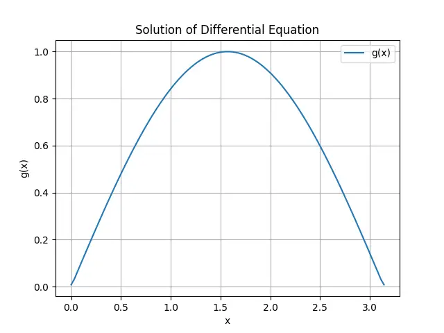
This example demonstrates how DST and its inverse can be utilized to solve a simple differential equation, showcasing the power of fft.dst() in scientific computing.

Conclusion

The fft.dst() function is an extraordinarily versatile tool in the domain of numerical computing. Whether you’re working with simple arrays, analyzing image data, manipulating higher-dimensional structures, or dealing with complex differential equations, fft.dst() provides a robust framework for frequency domain analysis. Through this tutorial’s progressive examples, we’ve barely scratched the surface of what’s possible with DSP and SciPy. Keep exploring, and you’ll find numerous applications of these principles in real-world scenarios.