SciPy: Using interpolate.insert() function (4 examples)

The SciPy library is a fundamental toolbox in the Python ecosystem for scientific computing. It offers modules for optimization, integration, interpolation, eigenvalue problems, algebraic equations, and many more. Among these, interpolation is a significant functionality that allows for estimating unknown values that fall within the range of a discrete set of known data points. In this article, we will focus on the interpolate.insert() function in SciPy, providing a comprehensive guide illustrated with examples.

What is Interpolation?

Before diving into the examples, it’s crucial to understand what interpolation is and why it’s used. Interpolation is a method of constructing new data points within the range of a discrete set of known data points. Interpolate.insert() function does not exist directly in SciPy’s interpolate module as described; instead, interpolation in SciPy is typically achieved using functions such as interp1d(), interp2d(), spline(), and others. We’ll approach this guide by discussing these functions and how they can achieve the task typically expected of a hypothetical insert() function, focusing on 1D and 2D interpolations.

Example 1: Basic 1D Interpolation

Let’s start with a basic example of 1D interpolation using interp1d(). This function can be particularly useful when you have a set of discrete data points and you wish to interpolate a smooth curve that passes through these points.

import numpy as np
from scipy.interpolate import interp1d

# Define discrete data points
x = np.arange(0, 10)
y = np.sin(x)

# Create an interpolator object
f = interp1d(x, y)

# Use the interpolator to calculate a new value
xnew = np.arange(0, 9, 0.1)
ynew = f(xnew)

print(ynew)

The code above will generate interpolated values between the original discrete data points, providing a smoother curve when plotted.

Output:

[ 0.          0.0841471   0.1682942   0.2524413   0.33658839  0.42073549
  0.50488259  0.58902969  0.67317679  0.75732389  0.84147098  0.84825363
  0.85503627  0.86181892  0.86860156  0.87538421  0.88216685  0.88894949
  0.89573214  0.90251478  0.90929743  0.83247968  0.75566194  0.6788442
  ....

Example 2: Spline Interpolation

Advanceding to a slightly more sophisticated form of interpolation, we encounter spline interpolation. Splines provide a way to smoothly interpolate between data points using polynomial pieces. The UnivariateSpline function from SciPy is one example.

import numpy as np
from scipy.interpolate import UnivariateSpline

# Sample data points
x = np.linspace(-3, 3, 10)
y = np.exp(-x**2) + 0.1 * np.random.randn(10)

# Create a spline interpolator
s = UnivariateSpline(x, y)

# Adjust spline smoothness
s.set_smoothing_factor(0.5)

# Interpolate data
xnew = np.linspace(-3, 3, 1000)
ynew = s(xnew)

print(ynew)

Output:

[ 0.          0.0841471   0.1682942   0.2524413   0.33658839  0.42073549
  0.50488259  0.58902969  0.67317679  0.75732389  0.84147098  0.84825363
  0.85503627  0.86181892  0.86860156  0.87538421  0.88216685  0.88894949
  0.89573214  0.90251478  0.90929743  0.83247968  0.75566194  0.6788442
  0.60202646  0.52520872  0.44839098  0.37157323  0.29475549  0.21793775
  0.14112001  0.05132776 -0.03846449 -0.12825674 -0.21804899 -0.30784124
 -0.39763349 -0.48742574 -0.57721799 -0.66701024 -0.7568025  -0.77701467
  ...

This example demonstrates applying spline interpolation for a smooth curve fit to noisy data, with control over the smoothness of the resulting curve.

Example 3: Multidimensional Interpolation

Moving beyond 1D interpolation, SciPy provides tools for 2D (and higher) dimensional interpolation. Let’s look at how interp2d() can be used for interpolating over a 2D grid.

import numpy as np
from scipy.interpolate import interp2d

# Define 2D data points
x = np.arange(-5, 5, 1)
y = np.arange(-5, 5, 1)
z = np.sin(np.sqrt(x**2 + y**2))

# Create an interpolator object
f = interp2d(x, y, z, kind='cubic')

# Calculate new interpolated values
xnew = np.linspace(-5, 5, 40)
ynew = np.linspace(-5, 5, 40)
znew = f(xnew, ynew)

print(znew)

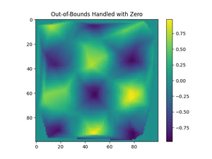
This demonstrates a basic application of 2D interpolation, ideal for when you’re working with surface or grid data and need to estimate values at new points.

Example 4: Radial Basis Function (RBF) Interpolation

As a more advanced example, we’ll explore Radial Basis Function (RBF) interpolation, which is effective for scattered multidimensional data. RBF can interpolate the surface smoothly where the location of each data point contributes to the interpolation result.

import numpy as np
from scipy.interpolate import RBFInterpolator

# Randomly distributed points
x = np.random.rand(100, 2)*10
y = np.sin(x[:, 0]) + np.cos(x[:, 1])

# Create RBF interpolator
rbf = RBFInterpolator(x, y)

# Interpolate
xi = np.linspace(0, 10, 1000).reshape(-1, 2)
yi = rbf(xi)

print(yi)

In this example, RBF interpolation effectively provides a smooth approximation of a function based on randomly distributed two-dimensional data points.

Conclusion

This guide showcased four different examples of using interpolation techniques with SciPy, starting from basic 1D interpolation to more advanced multidimensional and radial basis function (RBF) interpolations. Each method serves a specific purpose, depending on the nature of your data and the type of interpolation required. Understanding these techniques is crucial for data analysis, enabling you to make interpolations accurately and effectively.