SciPy fft.ifftshift() function (4 examples)

The SciPy library, an essential tool in the Python ecosystem, is widely recognized for its applications in mathematics, engineering, and scientific computing. Specifically, the Fast Fourier Transform (FFT) module within SciPy offers a myriad of functionalities for tackling complex numerical computations. Among these, the ifftshift() function plays a vital role, particularly in signal and image processing domains. This guide aims to demystify the ifftshift() function through a series of examples, progressively increasing in complexity.

Understanding fft.ifftshift()

Before diving into examples, it’s pivotal to grasp what ifftshift() does. Simply put, this function undoes the effect of fftshift(), which shifts the zero-frequency component to the center of the array. When applying FFTs for computational purposes, this shift enables a more intuitive frequency display. The ifftshift() function is thus employed to reverse this shift, commonly as a preparatory step before utilizing the inverse FFT (ifft()).

Example 1: Basic Usage

import numpy as np
from scipy.fft import ifftshift, fftshift

# Generating a simple array
arr = np.array([1, 2, 3, 4, 5])

# Applying fftshift to center the zero-frequency component
shifted_arr = fftshift(arr)

# Reversing the shift with ifftshift
restored_arr = ifftshift(shifted_arr)

print(restored_arr)

This code segment illustrates the fundamental operation of ifftshift(), where an initially shifted array is restored to its original configuration. The output will be:

[1 2 3 4 5]

Example 2: 2D Array Shift

In the realm of image processing, handling 2D arrays is common. Let’s examine how ifftshift() can be applied to a two-dimensional scenario.

import numpy as np
from scipy.fft import ifftshift, fftshift

# Create a 2D array
arr_2d = np.array([[1, 2, 3], [4, 5, 6], [7, 8, 9]])

# Apply fftshift
shifted_2d = fftshift(arr_2d)

# Reverse with ifftshift
restored_2d = ifftshift(shifted_2d)

print(restored_2d)

The output mirrors the original array, demonstrating the function’s applicability to multi-dimensional data:

[[1 2 3]
 [4 5 6]
 [7 8 9]]

Example 3: Real-world Signal Processing

Switching our focus to a practical application, consider a scenario in signal processing. Here, ifftshift() can significantly aid in aligning phases correctly before applying the inverse FFT.

import numpy as np
from scipy.fft import ifftshift, fftshift, ifft, fft

# Sample frequency (Hz)
f = 50

# Time vector (s)
t = np.linspace(0, 1, 500, endpoint=False)

# Generate a sampled sine wave
signal = np.sin(2 * np.pi * f * t)

# Apply FFT
signal_fft = fft(signal)

# Center the zero-frequency component
signal_fft_shifted = fftshift(signal_fft)

# Perform some processing (hypothetical)
# For illustration purposes, let's just copy it
processed_signal_fft_shifted = signal_fft_shifted.copy()

# Align phases correctly before IFFT
processed_signal_fft = ifftshift(processed_signal_fft_shifted)

# Apply inverse FFT
reconstructed_signal = ifft(processed_signal_fft)

print(np.allclose(signal, reconstructed_signal.real))

This example presupposes some frequency domain processing on a sine wave. The np.allclose() function is utilized to confirm that the inverse FFT reproduces the original signal accurately, considering minor numerical inaccuracies. The output, a boolean, signifies successful reconstruction:

True

Example 4: Advanced Image Processing

For our final example, let’s delve into complex image processing. In this scenario, ifftshift() functions to ensure spatial frequencies are accurately represented before applying inverse FFT.

import numpy as np
from scipy.fft import ifftshift, fftshift, ifft2, fft2
from matplotlib import pyplot as plt

# Load an image (this should be replaced with actual image loading in practice)
# Here, we simulate with a random array for illustration purposes
img = np.random.rand(256, 256)

# Convert to frequency domain
img_fft = fft2(img)

# Center the zero frequency
img_fft_shifted = fftshift(img_fft)

# Assuming some frequency domain processing (not shown)
# Reverse shift before IFFT
img_processed_fft = ifftshift(img_fft_shifted)

# Convert back to spatial domain
img_reconstructed = ifft2(img_processed_fft).real

# Display original and reconstructed image
plt.figure(figsize=(10, 5))
plt.subplot(121), plt.imshow(img, cmap='gray'), plt.title('Original Image')
plt.subplot(122), plt.imshow(img_reconstructed, cmap='gray'), plt.title('Reconstructed Image')
plt.show()

Output:

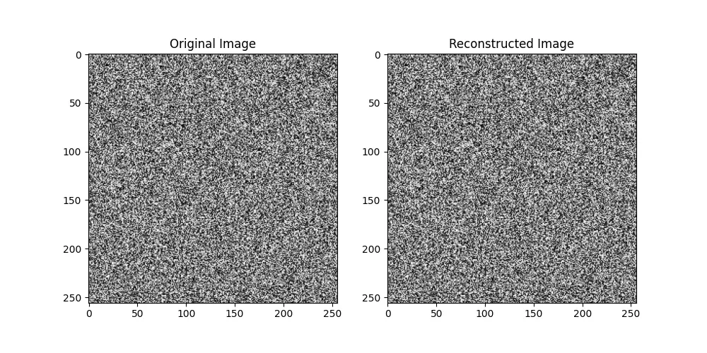
Although this example simulates image loading and processing, it illustrates the importance of ifftshift() in preparing images for accurate reconstruction post-processing in the frequency domain.

Conclusion

The ifftshift() function in SciPy’s FFT module is indispensable for applications requiring the reverse of zero-frequency component shifting. Through the gradual increase in example complexity, we explored its utility in array manipulation, signal, and image processing. Proper understanding and application of ifftshift() can significantly enhance the accuracy of inverse FFT operations, facilitating precise signal and image reconstruction.