SciPy cluster.hierarchy.complete() function (4 examples)

Clustering is a method of grouping sets of similar data points together. It’s a fundamental technique in data analysis and machine learning, enabling us to understand the natural groupings or structures within our data. The scipy.cluster.hierarchy module provides functions for hierarchical clustering, and among its various methods, the complete() linkage is a popular choice for many applications. This tutorial will explore the complete() linkage function in SciPy, illustrating its use through four progressively complex examples.

Introduction to complete() Linkage

In hierarchical clustering, the complete() linkage method considers the maximum pairwise distance between observations in two different clusters to determine the cluster distances. It’s also known as the farthest point algorithm. This strategy tends to find compact clusters of similar size. To utilize the complete() linkage clustering in SciPy, we use the complete() function from the cluster.hierarchy module.

Preparation

Before diving into examples, let’s prepare our environment:

import numpy as np
from scipy.spatial.distance import pdist, squareform
from scipy.cluster.hierarchy import complete, dendrogram
import matplotlib.pyplot as plt

With our environment set, we’re ready to explore some practical examples of using complete() linkage clustering.

Example 1: Basic Clustering

Let’s start with a simple example where we cluster a small dataset of points.

data = np.array([[0, 0], [1, 2], [3, 4], [5, 6]])
distance_matrix = pdist(data, 'euclidean')
Z = complete(distance_matrix)
dendrogram(Z)
plt.title("Dendrogram for Complete Linkage Clustering - SlingAcademy.com")
plt.show()

Output:

This example demonstrates how to compute the hierarchical clustering and display its dendrogram for a set of points. The dendrogram visualizes the sequence of merges that occur during clustering.

Example 2: Clustering with Custom Distance

Next, let’s explore how to use a custom distance metric for clustering.

def custom_metric(x, y):
    return np.linalg.norm(x-y)

data = np.array([[0, 1], [2, 3], [5, 6]])
distance_matrix = pdist(data, custom_metric)
Z = complete(distance_matrix)
dendrogram(Z)
plt.title("Custom Distance Dendrogram")
plt.show()

Output:

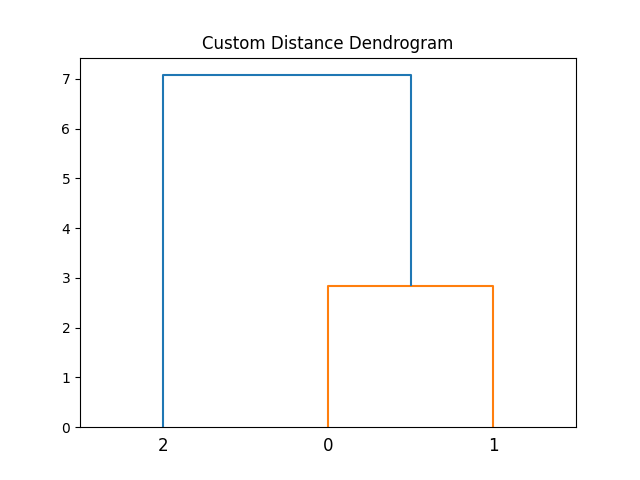
By defining a custom distance function, this example allows for more flexibility in how data similarities are calculated. This can be useful when the default distance metrics are not suitable for a particular dataset.

Example 3: Clustering Large Datasets

Clustering larger datasets presents additional challenges, mainly related to computational efficiency. Let’s see how to handle a more substantial set of points.

np.random.seed(2024)
data = np.random.rand(100, 2)
distance_matrix = pdist(data, 'euclidean')
Z = complete(distance_matrix)
dendrogram(Z)
plt.title("Large Dataset Dendrogram")
plt.show()

Output:

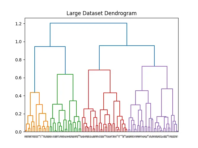
This example effectively demonstrates that the complete() linkage method, combined with efficient distance calculation strategies like pdist, can manage larger datasets.

Example 4: Advanced Visualizations and Clustering Insights

For an advanced example of using the scipy.cluster.hierarchy.complete() function for hierarchical clustering with insights and visualizations, let’s explore a scenario where we analyze and visualize a dataset to uncover clustering patterns. We’ll use the Iris dataset for this example due to its familiarity and ease of visualization, though the techniques can apply to more complex datasets.

Scenario: Iris Dataset Clustering with Complete Linkage

We aim to perform hierarchical clustering on the Iris dataset using the complete linkage method, then visualize the dendrogram and analyze the clustering results. We’ll also plot the clusters in the feature space for more insights.

Steps:

1. Load the Iris dataset.
2. Perform hierarchical clustering with complete linkage.
3. Visualize the dendrogram.
4. Extract cluster labels for a specific number of clusters.
5. Visualize the clusters in the feature space.

Implementation:

import numpy as np
import matplotlib.pyplot as plt
from scipy.cluster.hierarchy import complete, dendrogram, fcluster
from sklearn.datasets import load_iris
from sklearn.decomposition import PCA

# Step 1: Load the Iris dataset
iris = load_iris()
X = iris.data
y = iris.target

# Step 2: Perform hierarchical clustering
Z = complete(X)

# Step 3: Visualize the dendrogram
plt.figure(figsize=(10, 8))
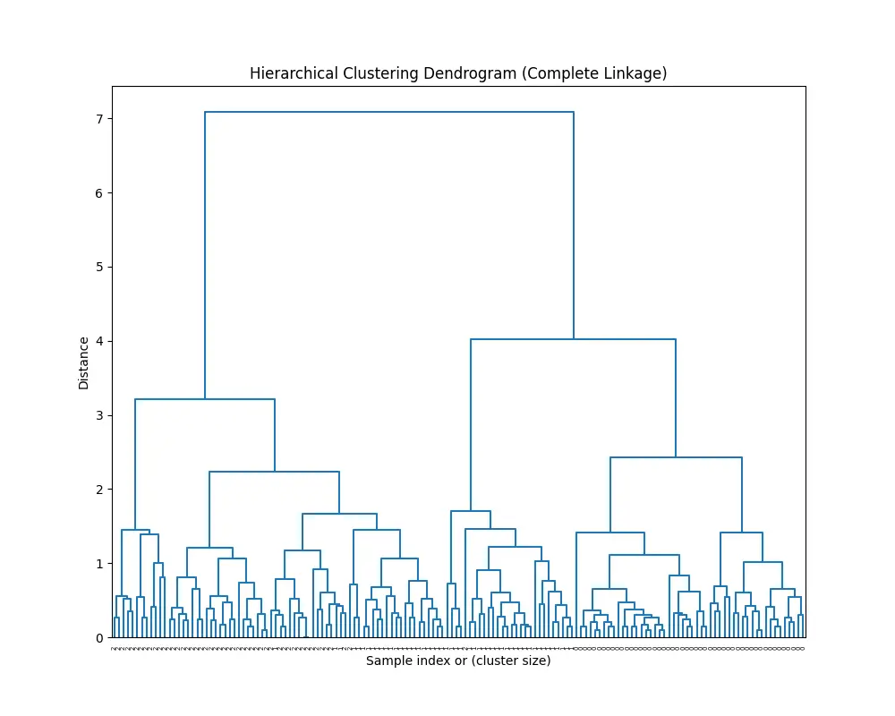
dendrogram(Z, labels=y, color_threshold=0)
plt.title('Hierarchical Clustering Dendrogram (Complete Linkage)')
plt.xlabel('Sample index or (cluster size)')
plt.ylabel('Distance')
plt.show()

# Step 4: Extract cluster labels
num_clusters = 3
cluster_labels = fcluster(Z, num_clusters, criterion='maxclust')

# Step 5: Visualize the clusters in the feature space
# For visualization, reduce dimensions to 2D using PCA
pca = PCA(n_components=2)
X_pca = pca.fit_transform(X)

plt.figure(figsize=(10, 8))
for i in range(1, num_clusters+1):
    plt.scatter(X_pca[cluster_labels == i, 0], X_pca[cluster_labels == i, 1], label=f'Cluster {i}')
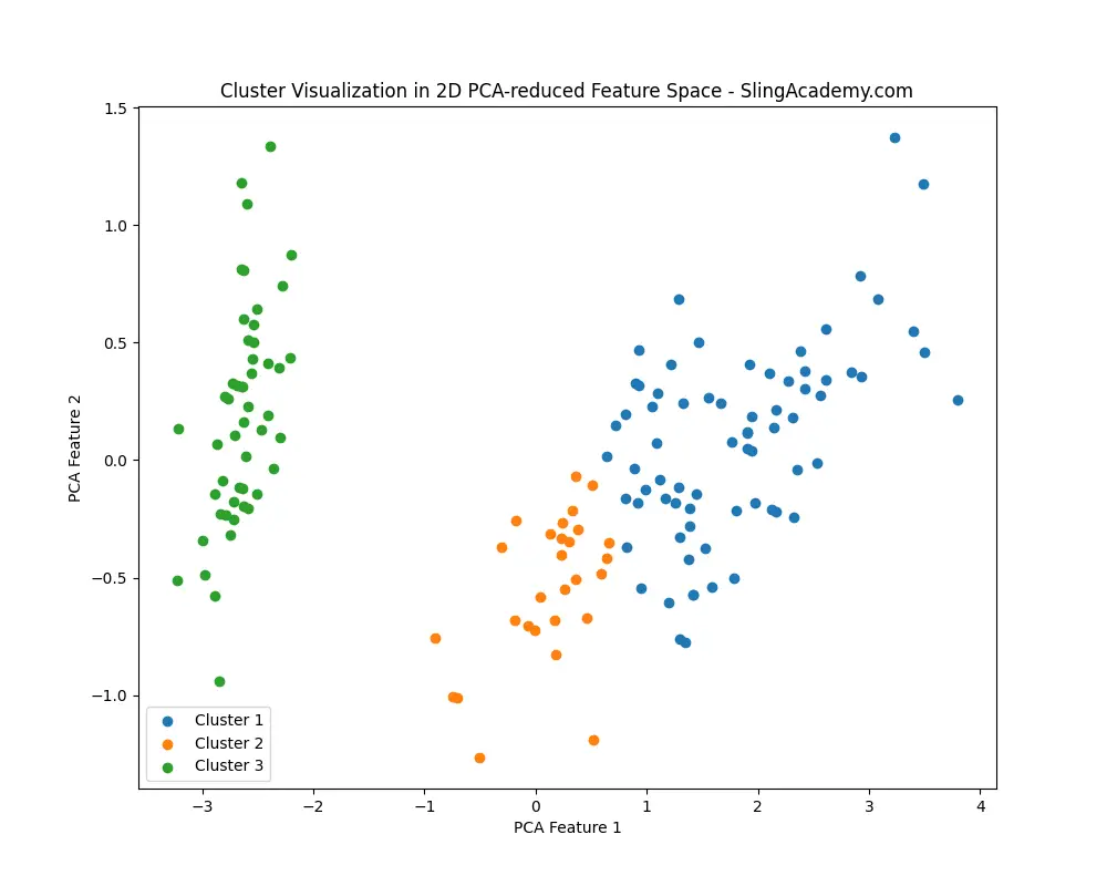
plt.title('Cluster Visualization in 2D PCA-reduced Feature Space - SlingAcademy.com')
plt.xlabel('PCA Feature 1')
plt.ylabel('PCA Feature 2')
plt.legend()
plt.show()

You’ll see this:

And this:

Conclusion

Through these examples, we’ve explored the versatility and power of the complete() linkage clustering method in SciPy’s hierarchical clustering module. Whether dealing with simple or more complex datasets, the complete() method offers a robust approach for identifying the natural groupings within data. By adjusting parameters and visualizations, we can gain a deeper understanding of our data’s structure, guiding more informed decision-making processes.