SciPy – Using cluster.hierarchy.fcluster() function (3 examples)

Clustering is a powerful tool in data science, enabling the identification of intrinsic groupings within data. One of the widely used methods for hierarchical clustering is provided by SciPy, a Python library that supports scientific and technical computing. In this guide, we will delve into the utilization of the fcluster() function from SciPy’s cluster.hierarchy module and illustrate its application with three progressive examples.

What does luster.hierarchy.fcluster() Do?

The fcluster() function in SciPy’s cluster.hierarchy module is designed for cutting hierarchical clusters to form flat clusters. This tutorial will explore its versatile options and applications through practical examples, from easy to complex scenarios, to grasp its functionality fully.

Getting Started

Before diving into the examples, ensure SciPy, NumPy, Matplotlib are installed in your environment. You can install them using pip:

pip install scipy numpy matplotlib

Once installed, you can import the necessary modules for our examples:

import numpy as np
from scipy.cluster.hierarchy import linkage, dendrogram, fcluster
import matplotlib.pyplot as plt

Example 1: Basic clustering

In our first example, we start with a simple dataset:

data = np.array([[5, 3], [10, 15], [15, 12], [24, 10], [30, 30], [
                85, 70], [71, 80], [60, 78], [70, 55], [80, 91],])

This example will demonstrate how to perform hierarchical clustering and use fcluster() to create flat clusters:

Z = linkage(data, 'ward')
plt.figure()
dendrogram(Z)
plt.show()
clusters = fcluster(Z, 2, criterion='maxclust')
print(clusters)

Output:

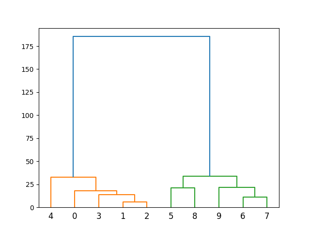
The output indicates the assignment of each data point to one of the two clusters.

The complete code for this example:

import numpy as np
from scipy.cluster.hierarchy import linkage, dendrogram, fcluster
import matplotlib.pyplot as plt

data = np.array([[5, 3], [10, 15], [15, 12], [24, 10], [30, 30], [
                85, 70], [71, 80], [60, 78], [70, 55], [80, 91],])

Z = linkage(data, 'ward')
plt.figure()
dendrogram(Z)
plt.show()
clusters = fcluster(Z, 2, criterion='maxclust')
print(clusters)

Example 2: Choosing a distance threshold

In this example, we illustrate the usage of a distance threshold for clustering instead of specifying the number of clusters:

import numpy as np
from scipy.cluster.hierarchy import linkage, dendrogram, fcluster

data = np.array([[5, 3], [10, 15], [15, 12], [24, 10], [30, 30], [
                85, 70], [71, 80], [60, 78], [70, 55], [80, 91],])

Z = linkage(data, 'ward')
clusters = fcluster(Z, 10, criterion='distance')
print(clusters)

Output:

[3 1 1 2 4 5 7 8 6 9]

This approach allows for more organic grouping based on the distances between points, resulting in clusters determined by the specified threshold.

Example 3: Advanced usage with custom distance metrics

For a more advanced scenario, consider we have a custom distance metric. This example shows how to use a precomputed distance matrix with fcluster() to perform clustering:

from scipy.spatial.distance import pdist
import numpy as np
from scipy.cluster.hierarchy import linkage, dendrogram, fcluster

data = np.array([[5, 3], [10, 15], [15, 12], [24, 10], [30, 30], [
                85, 70], [71, 80], [60, 78], [70, 55], [80, 91],])

Y = pdist(data, 'euclidean')
Z = linkage(Y, 'ward')
clusters = fcluster(Z, 5, criterion='maxclust')
print(clusters)

Output:

[1 1 1 1 2 3 4 4 3 5]

This method offers flexibility when dealing with complex data and custom definitions of distance.

Conclusion

Through these examples, we’ve demonstrated the versatility and utility of SciPy’s fcluster() function in the realm of hierarchical clustering. Starting with simple applications and moving to more sophisticated scenarios, we’ve seen how fcluster() provides the tools to create both straightforward and complex cluster solutions. With practice, you can leverage these insights to analyze and interpret your own data. Remember, the beauty of hierarchical clustering lies in its flexibility and depth, revealing the underlying structure of data in a way that is both informative and visually compelling.