NumPy random.Generator.standard_exponential() method (6 examples)

Introduction

NumPy, the fundamental package for scientific computing in Python, provides extensive functionality for generating random numbers. One of its features, the random.Generator.standard_exponential() method, allows users to draw samples from a standard exponential distribution, which has a mean of 1 and a variance of 1. This tutorial will explore six practical examples of using this method, progressively diving into its capabilities from basic to advanced uses.

Understanding standard_exponential()

This method is part of the newer numpy.random.Generator class, which aims to improve upon and eventually replace the older numpy.random.RandomState. It offers a stronger foundation for generating random numbers, supporting a wide range of distributions, including the standard exponential distribution.

Example 1: Basic Usage

To begin, let’s explore the simplest form of generating standard exponential samples:

import numpy as np

rng = np.random.default_rng()  # Create a Generator object
sample = rng.standard_exponential()
print(sample)

A possible output (vary):

0.23583425682501105

This code snippet will generate a single random sample from a standard exponential distribution. While the output is random, you can expect it to be a float value greater than zero.

Example 2: Generating Multiple Samples

Next, we’ll look at generating multiple samples at once, which is as simple as passing an argument to the method:

import numpy as np

rng = np.random.default_rng()
samples = rng.standard_exponential(5)  # Generate 5 samples
print(samples)

This will output an array of five random samples from the standard exponential distribution. This is particularly useful for simulations or modeling when you need a series of random values.

A possible output:

[0.03904371 2.19447427 6.35808444 2.77569796 0.01242453]

Example 3: Plotting the Distribution

Understanding the shape and characteristics of the exponential distribution can be achieved through visualization using matplotlib:

import numpy as np
import matplotlib.pyplot as plt

rng = np.random.default_rng()
samples = rng.standard_exponential(1000)

plt.hist(samples, bins=30, density=True)
plt.title('Standard Exponential Distribution')
plt.xlabel('Value')
plt.ylabel('Frequency')
plt.show()

Output (random):

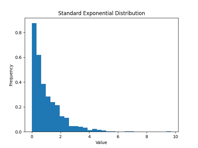
This histogram plots 1000 samples, providing a visual representation of the distribution’s characteristics. It’s clear that most values cluster near zero, with frequency decreasing as values increase, which is typical of an exponential distribution.

Example 4: Reproducibility with Seeds

For many applications, it’s essential to produce the same set of random numbers, which can be achieved by setting a seed:

import numpy as np

seed = 42
rng = np.random.default_rng(seed)
samples = rng.standard_exponential(5)
print(samples)

Output:

[2.4042086  2.33618966 2.384761   0.27979429 0.0864374 ]

This will generate a deterministic output, meaning you’ll get the same five numbers each time this code is run. Reproducibility is crucial in scientific research, testing, and debugging.

Example 5: Advanced Simulation

Utilizing the standard_exponential() function in simulations or models can provide insight into processes with exponential timing, such as service times in a queue system:

import numpy as np

rng = np.random.default_rng(seed=2024)
service_times = rng.standard_exponential(100)
queue_lengths = [service_times[:n].sum() for n in range(1, 101)]

# Simulate queue length over time
print(queue_lengths[-1])

Output:

85.39105469125145

This simulates the total service time for 100 consecutive customers. The resulting list, queue_lengths, represents the cumulative service time. This can illustrate, for example, how long a queue becomes over time as more customers are served, each with a service time drawn from a standard exponential distribution.

Example 6: Integration with Other Distributions

Finally, the standard_exponential() method can be combined with other distribution samplings to model complex systems. For example, using both normal and exponential distributions to simulate real-world random events:

import numpy as np

rng = np.random.default_rng(seed=2024)
arrival_times = rng.standard_exponential(100)
service_times = rng.normal(loc=3, scale=1, size=100)

# Calculate total time
total_times = arrival_times + service_times
print(total_times)

Output:

[3.80364892 2.7843935  2.64980168 6.61610126 2.85771297 3.21164454
 3.58819007 3.90166454 1.48467145 3.55414346 1.89353181 3.30892467
 3.91634073 3.16598957 2.91997158 7.80575111 6.35477478 3.88196298
 3.48704753 1.28743001 5.25826633 4.98105307 3.20387174 2.48723807
 3.38558468 6.45315559 4.29970231 3.90785476 2.68594607 4.10814153
 0.28562034 3.01200414 3.07518346 2.38152766 3.0784992  4.03747654
 4.09550388 3.47416505 5.00507441 8.65668626 2.84302654 4.81171477
 3.00222647 3.35506001 3.21352198 3.72956817 3.75952343 3.22018636
 3.96688247 2.55155731 4.15714247 4.27183808 3.95617885 6.33498752
 4.18147254 5.12486472 3.34562383 6.94889161 5.07600075 7.97772992
 3.25321678 4.01447803 7.14275662 3.28387504 3.92358322 3.83305044
 1.74346284 2.36170855 4.14815034 4.32253395 5.17725215 3.03124507
 1.15710201 4.94011443 3.05085487 1.36616138 1.32388247 2.24288295
 3.64623098 3.96790505 3.9202586  3.90170638 3.61836035 4.04269122
 3.71143606 2.65338405 4.98763654 1.70471571 3.3629379  2.42933126
 5.13019636 1.81355197 4.33671369 2.27519512 1.62735136 2.9983412
 5.62739262 2.89008321 2.16515153 3.72794151]

This approximates a scenario where entities have both a random arrival time (exponentially distributed) and a random service time (normally distributed), typical in customer service or networking models.

Conclusion

The standard_exponential() method in NumPy’s random generation suite is a powerful tool for simulating and understanding random processes with exponential characteristics. From basic single-value generation to complex simulations involving multiple distributions, it provides a venue for exploring and analyzing randomness in scientific computing. As we’ve seen through these examples, whether you’re involved in data science, engineering, or analytics, mastering this functionality can greatly enhance your modeling and simulation capabilities.