Introduction
The fft.fftshift() function in SciPy is a powerful tool for signal processing, particularly in the context of Fourier transforms. It allows for the rearrangement of Fourier Transform outputs into a zero-frequency-centered spectrum, making analysis more intuitive and insightful.
Background on the Fourier Transform and fft.fftshift()
The Fourier Transform is a mathematical technique used to convert signals from time or space domain to frequency domain. In context, the fft() function in SciPy computes the Discrete Fourier Transform (DFT). The result of a DFT on real-world data can be challenging to interpret, mainly because the output frequencies are arranged in a mix of positive and negative frequencies. This is where fft.fftshift() steps in, as it shifts the zero-frequency component to the center of the array, which is especially useful for visualization and further processing. The function ifftshift() is its inverse, used to shift back for inverse transformations.
Basic Example
Let’s begin with a basic example to illustrate how fft.fftshift() works:
import numpy as np
from scipy.fft import fft, fftshift

# Generate a simple signal
x = np.linspace(0, 2*np.pi, 128)
y = np.sin(x)

# Compute the FFT
Y = fft(y)

# Shift the FFT
Y_shifted = fftshift(Y)

# Compare
print(Y[0:5]) # Original FFT output
print(Y_shifted[0:5]) # After fftshift
Output:
[-4.02455846e-16 -0.j          1.56431722e+00-63.72321906j
 -3.31505794e-02 +0.67479555j -2.78784933e-02 +0.37793951j
 -2.64085428e-02 +0.26813044j]
[-0.024742  -0.j         -0.02474201-0.00060738j -0.02474203-0.0012155j
 -0.02474208-0.00182509j -0.02474214-0.00243689j]
In the code above, we start by generating a simple sine wave, then we compute its FFT and apply fft.fftshift(). The printed outputs demonstrate how the zero-frequency component is repositioned towards the center of the array after shifting.
Intermediate Example
For a more detailed example, let’s analyze how fft.fftshift() benefits in the visualization of the spectrum of a more complex signal:
import numpy as np
import matplotlib.pyplot as plt
from scipy.fft import fft, fftshift

# Generate a complex signal
sample_rate = 1000
T = 1/sample_rate
t = np.linspace(0, 1.0, int(1/T), endpoint=False)
y = np.sin(50 * 2 * np.pi * t) + 0.5 * np.sin(80 * 2 * np.pi * t)

# Compute and shift FFT
Y = fft(y)
Y_shifted = fftshift(Y)
xf = np.linspace(-sample_rate/2, sample_rate/2, len(y))

# Plot
plt.figure()
plt.plot(xf, np.abs(Y_shifted))
plt.title('Shifted Frequency Spectrum')
plt.xlabel('Frequency (Hz)')
plt.ylabel('Magnitude')
plt.show()
Output:
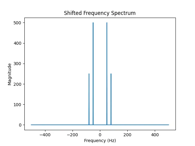
The above code generates a complex signal by combining sinusoidal waves and displays its frequency spectrum. By employing fft.fftshift(), the frequency components are illustrated with zero frequency in the center, providing a clearer perspective on the signal’s composition.
Advanced Example
Finally, let’s delve into a more sophisticated scenario involving image processing. In this example, we apply fft.fftshift() to interpret the frequency domain representation of an image:
import numpy as np
import matplotlib.pyplot as plt
from scipy.fft import fft2, fftshift
from scipy.datasets import ascent # Sample image

# Load sample image
image = ascent()

# Compute 2D FFT and shift
F_image = fft2(image)
F_image_shifted = fftshift(F_image)

# Display the magnitude spectrum
plt.figure()
plt.imshow(np.abs(F_image_shifted), cmap='gray')
plt.title('Shifted Frequency Spectrum of Image')
plt.colorbar()
plt.show()
Output:
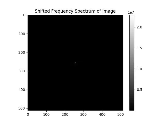
In this advanced example, we process a 2D signal (an image) and shift its Fourier transform, revealing the frequency components neatly centered. This technique is particularly relevant in fields like medical imaging, astronomy, and computer vision, where understanding the frequency content of an image is crucial.
Conclusion
The fft.fftshift() function in SciPy is an invaluable asset in the arsenal of data analysts and researchers dealing with signals and images. Through the examples provided, we can appreciate how shifting the zero-frequency element to the center of a Fourier Tranform’s output array enriches our understanding and facilitates a more refined analysis. As we explored, from basic signal processing to advanced image analysis, fft.fftshift() opens up possibilities for insights that might otherwise remain obscured in the unshifted frequency domain.