SciPy – Working with interpolate.splrep() function (4 examples)

The SciPy library is a core part of the Python ecosystem, offering a vast array of modules for mathematics, science, and engineering. Within the SciPy framework, the interpolate.splrep() function is a powerful tool for creating smooth spline representations of data. This tutorial delves into the splrep() function, guiding you through four progressively advanced examples of how to use it effectively.

What does splrep() Do?

The splrep() function from the scipy.interpolate module calculates the B-spline representation of a 1-dimensional curve. Unlike many interpolation methods that fit a global function to data, B-splines approximate the curve with a piecewise polynomial function which offers greater flexibility and smoothness.

Example 1: Basic Spline Representation of Linear Data

To start with the most basic example, let’s create a linear set of data points and use splrep() to compute the spline representation.

import numpy as np
from scipy.interpolate import splrep, splev

# Generate linear data
x = np.linspace(0, 10, 10)
y = 2 * x + 5

# Calculate the spline representation (knots, coefficients, and degree)
tck = splrep(x, y, s=0)

# Use splev to evaluate the spline at a set of points
x_new = np.linspace(0, 10, 100)
y_spline = splev(x_new, tck)

# Plot the original and spline-interpolated data
import matplotlib.pyplot as plt

plt.figure(figsize=(8, 6))
plt.plot(x, y, 'o',  label='Original Data')
plt.plot(x_new, y_spline, '-', label='Spline Fit')
plt.legend()
plt.show()

Output:

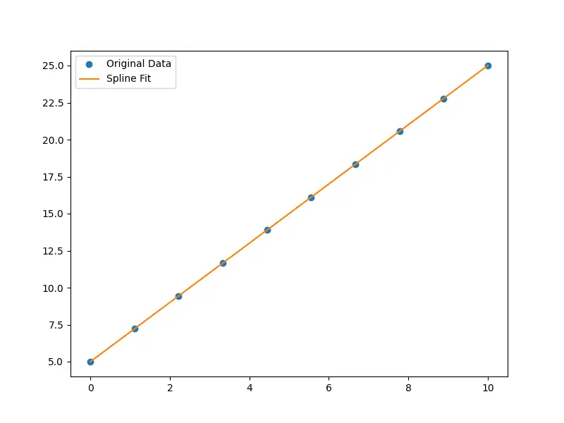
In this example, the output is a visual comparison between the original data and its B-spline representation, illustrating how splrep() smoothly interpolates between data points.

Example 2: Handling Non-linear Data

Building upon the initial example, let’s consider a non-linear set of data points and observe how splrep() manages more complex curves.

import numpy as np
from scipy.interpolate import splrep, splev
import matplotlib.pyplot as plt

# Generate non-linear data
x = np.arange(0, 10, 0.5)
y = np.sin(x)

# Calculate the spline representation
s=0
tck = splrep(x, y)

# Evaluate the spline over a finer grid
x_new = np.linspace(0, 10, 200)
y_spline = splev(x_new, tck)

# Visualize the fit
plt.figure(figsize=(8, 6))
plt.plot(x, y, 'o', label='Original Data')
plt.plot(x_new, y_spline, '-', label='Spline Fit')
plt.legend()
plt.show()

Output:

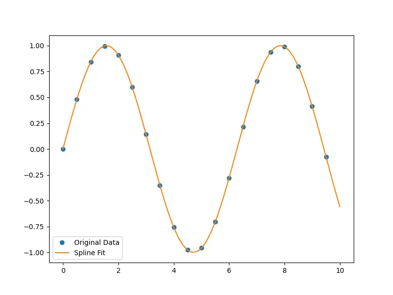
This example demonstrates the capability of splrep() to faithfully represent non-linear relationships, offering a smooth curve that approximates the original sinusoidal data effectively.

Example 3: Weighted Data Fitting

One notable feature of the splrep() function is the ability to apply weights to the data points, prioritizing the fit in certain areas over others. This is particularly useful when dealing with data of varying reliability.

import numpy as np
from scipy.interpolate import splrep, splev
from matplotlib import pyplot as plt

# Generate noisy non-linear data
x = np.arange(0, 10, 0.5)
y = np.sin(x) + np.random.normal(0, 0.1, len(x))

# Define weights – higher values give greater emphasis
c = np.linspace(1, 5, len(x))

# Calculate the spline with weighted data
s=0
tck = splrep(x, y, w=c)

# Evaluate and plot
x_new = np.linspace(0, 10, 200)
y_spline = splev(x_new, tck)

plt.figure(figsize=(8, 6))
plt.plot(x, y, 'o', label='Original Data')
plt.plot(x_new, y_spline, '-', label='Weighted Spline Fit')
plt.legend()
plt.show()

Output:

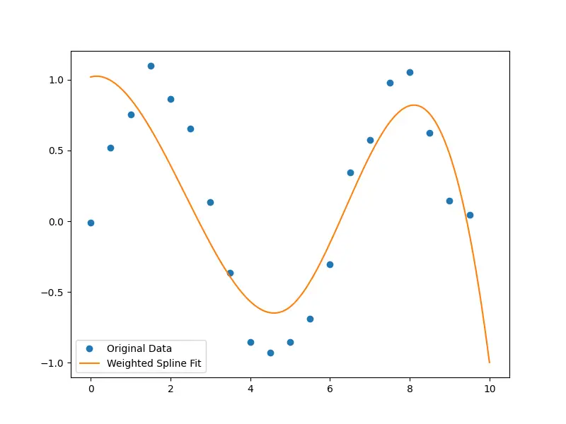
The output should display a refined spline curve that gives precedence to later (presumably more accurate) data points, illustrating how weights can influence the fitting process.

Example 4: Specifying Spline Smoothness

The smoothing factor (s) parameter in splrep() allows users to control the trade-off between closeness of fit and smoothness of the spline curve. Let’s explore its effects with an example.

import numpy as np
from scipy.interpolate import splrep, splev
from matplotlib import pyplot as plt

# Generate noisy data
x = np.linspace(0, 10, 10)
y = np.sin(x) + np.random.normal(0, 0.2, len(x))

# Calculate the spline with different smoothing factors
tcks = [splrep(x, y, s=i) for i in [0, 1, 10]]

# Evaluation
x_new = np.linspace(0, 10, 100)
plots = plt.figure(figsize=(10, 8))
labels = ['s=0', 's=1', 's=10']
for tck, label in zip(tcks, labels):
    y_spline = splev(x_new, tck)
    plt.plot(x_new, y_spline, '-', label=label)
plt.plot(x, y, 'o', label='Original Data')
plt.legend()
plt.show()

Output:

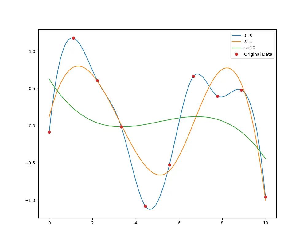
This visual comparison allows you to see how varying the smoothing factor can either produce a curve that closely fits the data (at the risk of overfitting) or a smoother curve that may underfit but provides a gentler overall trend.

Conclusion

The splrep() function in SciPy’s interpolation module is a versatile tool for smoothing and interpolating data. Through these examples, we’ve seen how it can adjust to linear and non-linear data, incorporate weighting, and balance the trade-off between fit and smoothness. With splrep(), Python offers a powerful method for sophisticated data analysis and visualization.